High-precision blood glucose prediction and hypoglycemia warning based on the LSTM-GRU model

Objective: The performance of blood glucose prediction and hypoglycemia warning based on the LSTM-GRU (Long Short Term Memory - Gated Recurrent Unit) model was evaluated.

Methods: The research objects were 100 patients with Diabetes Mellitus (DM) who were chosen from Henan Provincial People’s Hospital. Their continuous blood glucose curves of 72 hours were acquired by a Continuous Glucose Monitoring System (CGMS). The blood glucose levels were predicted based on the LSTM, GRU and LSTM-GRU models, respectively. Analyses of the best predictive model were performed using Root Mean Square Error (RMSE), Mean Absolute Percentage Error (MAPE), Mean Absolute Error (MAE) and correlation analysis between the prediction blood glucose level and the original blood glucose level acquired by CGMS and Clark Error Grid Analysis (EGA). Repeated-measures analysis of variance (ANOVA) was used to analyze whether the RMSE values of the three models were statistically significant. 60 patients who had experienced hypoglycemia among 100 cases were selected for hypoglycemia warning. The sensitivity, false-positive rate and false-negative rate were used to evaluate the hypoglycemia warning performance of the LSTM-GRU model. This paper explored the changing relationship of the hypoglycemia warning performance of the model over time.

Results: The predicted blood glucose levels of the three models were strongly correlated with the blood glucose levels acquired by CGMS (p < 0.001). The correlation coefficient (R-value) of the LSTM-GRU model remained sover time (R = 0.995), nevertheless, a reduction in the R-value of the LSTM and GRU models when the Prediction Horizon (PH) was 30 min or longer. When PH was 15min, 30min, 45min and 60min, the mean RMSE values of the LSTM-GRU model were 0.259, 0.272, 0.275 and 0.278 (mmol/l), respectively, which were lower than the LSTM and GRU models and the RMSE values were statistically significant (p < 0.001). The EGA results showed the LSTM-GRU model had the highest proportion in zones A and B, as the PH extended. When PH was 30min or longer, the sensitivity and false-negative rate of the hypoglycemia warning of the LSTM-GRU model had subtle changes and the false-positive rate remained sover time.

Conclusions: The LSTM-GRU model demonstrated good performance in blood glucose prediction and hypoglycemia warning.

Introduction

Diabetes mellitus (DM) is a group of chronic metabolic conditions, all of which are characterized by elevated blood glucose levels resulting from the body’s inability to produce insulin or resistance to insulin action, or both [1]. Blood glucose levels that are too high or too low can cause a series of diabetes-related complications [2-4].

With the progress of blood glucose monitoring technology, the clinical application of a continuous glucose monitoring system (CGMS) is gradually popularized. CGMS is a blood glucose monitoring system, which is designed to continuously monitor interstitial fluid (ISF) glucose levels within a range of 40-400 mg/dl [5]. The CGMS is consisted of a disposable sensor inserted into the subcutaneous tissue, taches to a sensor and receiver that displays and stores glucose data [6] and can obtain complete blood glucose levels fluctuation curve by converting glucose concentration in ISF to blood glucose levels. Therefore, CGMS can be used to assess blood glucose levels comprehensively and document more accurately the actual incidence of hypoglycemia and make it possible to develop blood glucose prediction models [7-8].

Blood glucose prediction models [9] mainly include data-driven blood glucose prediction models, physiological blood glucose prediction models and mixed-blood glucose prediction models. Physiological models [10] are usually built based on extensive knowledge and understanding of insulin, glucose metabolism and other parameters. Data-driven models [11] mainly rely on blood glucose measurements. Hybrid blood glucose prediction models [12] combine the two previous approaches together. Since physiological models are somewhat time-consuming and require prior knowledge to set physiological constants, data-driven blood glucose prediction models have gained popularity in recent years. Yang, et al. [13], proposed an autoregressive integral moving average (ARIMA) model with an adaptive recognition algorithm of model for blood glucose prediction and hypoglycemia warning. Sparacino, et al. [14], demonstrated a first-order autoregressive (AR) model to predict blood glucose levels, with a prediction horizon (PH) of 45min. Wang, et al. [15], proposed a new adaptive weighted average framework for blood glucose prediction algorithms, of which the main idea was to give each algorithm an adaptive weight, where the weight of each algorithm was inversely proportional to the sum of squared prediction errors. The method achieved satisfactory results for blood glucose prediction and it had very strong robustness to changes in patients and PHs. Pérez-Gandía, et al. [16], used an Artificial Neural Network (ANN) model based on CGMS data. Fernandez, et al. [17], used an artificial neural network to predict blood glucose levels based on patient dynamics, CGMS measurements, and insulin doses. Wang, et al. [18], proposed a short-term blood glucose prediction model combining variational mode decomposition (VMD) and an improved Particle swarm optimization optimizing long short-term memory network (IPSO-LSTM) and the model had high prediction accuracy even when PH was extended to 60min. In general, the more accuracy of blood glucose prediction and the longer PH can provide clinicians and patients with sufficient time to prevent hypoglycemia events.

With the development of information technology, more and more machine learning algorithms are introduced in the field of blood glucose prediction, such as Long Short-Term Memory (LSTM) [19,20] and GRU [21]. Due to the working principles of the LSTM and GRU being similar and these two models being deficient in each other, this paper proposed a composite model for blood glucose levels prediction and hypoglycemia warning.

The structure is set as follows: In the first part, an introduction to the basic principle of the three models is carried out. The second part introduces the experimental dataset and the process followed to develop a set of indicators that are evaluated in this paper. The third part presents the experimental results. The fourth part gives the discussion. And the last part provides conclusions of the paper and outlines directions for future research.

Modeling principle

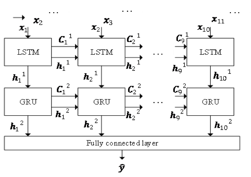
To predict blood glucose levels, a combination model was proposed, illustrated in Figure 1. It contains an LSTM layer, a GRU layer and a fully connected layer. Take several blood glucose values as input and train through LSTM and GRU. A fully connected layer to output the predicted level.

Figure 1: Principle of the combinational model.

The first layer is the LSTM layer, illustrated in Figure 2, consisting of a forget gate f_t, an input gate i_t and an output gate o_t. The forget gate decides what information to discard. The input gate determines what information is inputted to the cell state. The calculating process in LSTM cells is as follows.

Figure 2: Principle of the LSTM.

$f_t=\text{σ}(W_f\times \left[h_{t-1},x_t\right]+b_f)$

$i_t=\sigma (W_i\cdot \left[h_{t-1},x_t\right]+b_i)$

${\tilde{C}}_t=\tanh \left(W_c\cdot \left[h_{t-1},x_t\right]\right)+b_c$

$C_t=f_t\text{*}{C}_{t-1}+i_t\text{*}{\tilde{C}}_t$

Where the xt is input and h_t-1 is the hidden state of the previous moment. W, b represent the weights matrix and biases vector, respectively and Ct-1 is the cell state of the previous moment. In addition, h_t-1 is hidden state of the previous moment and is candidate cell state.

The h_t-1 and x_t are activated by the sigmoid function of the output gate to obtain o_t and the new cell state is activated by the tanh function to update the hidden state h_t.

$o_t=\sigma (W_o\cdot \left[h_{t-1},x_t\right]+b_o)$

$h_t=o_t*\tanh (C_t)$

W_f, W_i, W_c, W_o and b_f, b_i, b_c, b_o are parameters of the model and can be learned.

The above content is the calculation process of the LSTM and its entire network follows the rules of backpropagation and gradient descent to update parameters. This structure can effectively screen the effective features of long-term data and solve the long-dependency problem of the RNN (recurrent neural network).

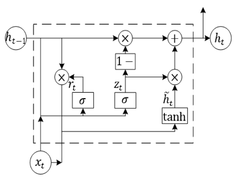
The second layer is the GRU unit, illustrated in Figure 3. The two gates of the GRU are called the reset gate r_t and the update gate z_t . r_t determines how much of the secret state at the last moment is retained and how much is reset. z_t is used to control the degree to which the state information of the previous moment is brought into the current state. The updated formula is as follows.

Figure 3: Principle of the GRU

$r_t=\sigma (W_r\cdot \left[h_{t-1},x_t\right])$

$z_t=\sigma (W_z\cdot \left[h_{t-1},x_t\right])$

${\tilde{h}}_t=\text{tanh}(W_{{\tilde{h}}_t}\cdot \left[r_t*h_{t-1},x_t\right])$

$h_t=\left(1-z_t\right)\text{*}{h}_{t-1}+z_t*{\tilde{h}}_t$

Where ${\tilde{h}}_t$ is the candidate’s hidden state. W_r, W_z,$W_{{\tilde{h}}_t}$ are parameters of the model and can be learned.

Finally, extract all hidden states, make the final output hidden state $h_n=\{h_1,h_2,\dots ,h_t\}$ and then calculate with the output weight W_n and the output bias vector b_n to obtain the predicted value $\hat{y}$ .

$\hat{y}=W_n{h}_n+b_n$

Experiments

A. Dataset: The blood glucose curves of 100 patients with DM who received subcutaneous insulin infusion therapy during hospitalization in the Endocrinology Department of Henan Provincial People’s Hospital were retrospectively analyzed from March 2017 to December 2017. All patients met the World Health Organization (WHO) DM diagnostic criteria [22]. The following DM patients were excluded: DM patients with critically ill and unspatients, gestational diabetes, allergies, or a history of tape allergy, the wearing time is less than 72 hours and the original blood glucose levels sequence has a breakpoint.

B. Data preprocessing: The original CGMS data was nonlinear and non-stationary. firstly, we decomposed the original CGMS data using the sym5 wavelet transform [23], removed high-frequency signals, kept low-frequency signals and used a one-dimensional reconstruction function to obtain denoised blood glucose curves, illustrated in Figure 4. This method improved the validity of the original CGMS data and the accuracy of the model prediction, to some extent. Secondly, To get a better prediction effect, a min-max normalization was used to transform blood glucose levels to the range (0,1).

Figure 4: Wavelet denoising.

C. Performance evaluation: Correlation analysis was used to evaluate the degree of correlation between the predicted blood glucose level and the CGMS data. The greater the correlation, the better the prediction is. RMSE (Root Mean Square Error), MAPE (Mean Absolute Percentage Error) and MAE (Mean Absolute Error) [24], were used in this paper to evaluate the prediction performance of the LSTM, GRU and LSTM-GRU models. This paper took RMSE as a statistical indicator and repeated-measures analysis of variance (ANOVA) was used to compare the prediction performance between the three models and obtained the best predictive model.

Carrillo-Moreno, et al. [25], stated that the PH has to be long enough (at least 15min), so clinicians and patients have time to adjust their treatment. This paper compared three models with four different PHs: 15min, 30min, 45min and 60min.

The above statistical methods were all operated by the SPSS 26.0 and p < 0.05 was considered statistically significant.

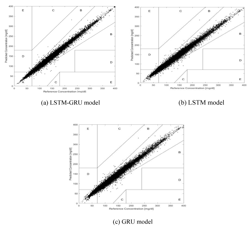
Clark Error Grid Analysis(EGA) [26]: Using the Beckman analyzer as the reference, the grid is subdivided into five zones: A, B, C, D and E. Values in zones A and B represent accurate or accepand values in Zone C, D and E represent error and the data is not desirable. The ISO15197:2013 standard [27], requires 99% of the blood glucose levels to fall within zones A and B.

D. hypoglycemia warning: The International Hypoglycaemia Study Group (IHSG) defines hypoglycemia as a measurable glucose concentration of 3.9mmol/l [28]. hypoglycemia warning means when the blood glucose level predicted in advance fall below the threshold of 3.9mmol/l, the model will trigger hypoglycemia alerts timely and notify clinicians and patients to take action to prevent hypoglycemia before it happens. TP, TN, FP and FN [29] were used to assess each of the indicators, which included sensitivity, false-positive and false-negative used to evaluate the performance of hypoglycemia warning. This paper explored the hypoglycemia warning performance with PH was extended.

Results

A. Pearson correlation analysis

The results of Pearson correlation analysis between the predicted blood glucose level of the three models and the original blood glucose level acquired by CGMS are shown in Table 1. For different PHs, the predicted blood glucose level of each model was positively correlated with the original blood glucose level acquired by CGMS (p < 0.001). The R - values (R = 0.995) of the LSTM-GRU model were identical when different PHs, nevertheless, a reduction in the LSTM and GRU model’s performance start to appear when PH was 30 min or longer.

B. Repeated-measures ANOVA

The prediction performance of 100 DM patients is shown in Table 2 and the results of the RMSE value variance analysis are provided in Table 3. When PH was 15min, 30min, 45min and 60min, the mean RMSE values of the LSTM-GRU model were 0.259, 0.272, 0.275 and 0.278 (mmol/l), respectively. The mean RMSE values of the LSTM-GRU model were lower than those of the LSTM and GRU models with identical PHs and had statistically different (p < 0.001), while the mean RMSE values of the LSTM and GRU models had no statistical significance (p > 0.05).

C. Clark error grid analysis

The EGA results of the three models are shown in Table 4 and Figure 5. Due to zones C, D and E being of little significance for clinical reference, it was not listed in Table 4

Figure 5: The EGA results of the three models (60min).

D. Results of hypoglycemia warning

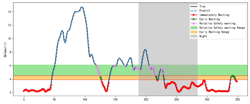
The hypoglycemia warning performance of 60 DM patients with hypoglycemia is shown in Table 5. When PH was 15min, 30min, 45min and 60min, the mean sensitivity were 91.21%, 89.71%, 89.21% and 88.73%, the mean false-negative rate were 8.79%, 10.29%, 10.79% and 11.27%, the mean false-positive rate were 0.88%, 0.90%, 0.87% and 0.87%. As the PH was extended, the results of the false-positive rate were almost identical, nevertheless, the sensitivity of the model gradually decreased, but the false-negative rate gradually increased and some differences in the model performance start to appear when the PH was 30min. The results of the statistical analysis of sensitivity are shown in Table 6. The sensitivity of the model with a PHs of 30min or longer had significant differences from the sensitivity of a PH of 15min (p < 0.05), while the sensitivity with a PHs of 30min, 45min and 60min had no difference (p > 0.05). This paper took patient B as an example and its warning result is shown in Figure 6.

Figure 6: Hypoglycemia warning figure (60min).

Discussion

The purpose of blood glucose control is to reach a normal concentration of blood glucose, minimizing the occurrences of hypoglycemia and hyperglycemia, respectively. Hypoglycemia can invoke dangerous situations, is feared by many patients with diabetes and is recognized as a key factor that can lead to failure to reach and maintain good glycemic control, repeated episodes of hypoglycemia can increase the incidence of diabetes-related complications [30]. Therefore, controlling the normal concentration of blood glucose with modern information technology is of great significance for reducing the occurrence of diabetes-related complications.

Based on both the LSTM and GRU models regulating information flow through gate mechanisms, the LSTM-GRU model in this paper was proposed. The results show that a PH of 15min had the highest accuracy and a reduction in prediction accuracy of the three models, as the PH was extended. However, the prediction errors of the three models were all within the acceprange. A PH of 15min is the most accurate, but they do not provide enough time for clinicians to take action when hypoglycemia happened and the models with a PHs of 30min or longer are good enough to allow a patient to do the necessary adjustments in insulin delivery and consequently to prevent the occurrence of hypoglycemia events. Theoretically, the longer PH, the higher the clinical value is. However, due to a reduction in prediction performance over time, the longest time was 60min in this paper.

Correlation analysis can be a good measure to evaluate the degree of correlation between the blood glucose level predicted by the model and the original blood glucose level acquired by CGMS. The results showed the R-values of the LSTM-GRU model were identical with different PHs (R = 0.995), while the R-values of the LSTM and GRU models started to reduce when PH was 30 min or longer, but all values had excellent correlations (R > 0.5, p < 0.001), which provided certain theoretical support for the LSTM-GRU model to be used for accurate long-term prediction. Zones A and B of the EGA represent the clinically accurate and accepzones, respectively. With different PHs, the proportion of the LSTM-GRU model in zones A and B was higher than in the LSTM and GRU models. That is, as the PH was extended, the blood glucose levels predicted by the LSTM-GRU model were closer to the original blood glucose level acquired by CGMS and the prediction effect was the best. The repeated-measures ANOVA results showed that RMSE values of the LSTM-GRU model had differences from the LSTM and GRU models with different PHs (p < 0.05), and RMSE values of the LSTM-GRU model were lower than the LSTM and GRU models with identical PHs. In summary, we can conclude that the LSTM-GRU model had the best prediction performance. The reason might be the structure of the LSTM-GRU model. The first layer is the LSTM unit, which inherits the learning advantages of the LSTM model in a longer time range. On this basis, The second layer was the GRU unit, which made the sample data easy to train and shortened the operation time. Finally, a fully connected layer (dense layer) was used to connect the hidden layer and the output layer. The LSTM-GRU model made up for the insufficiency of a single model, which improved the overall prediction performance of the model and prolonged the PH.

Based on the efficient prediction performance of the LSTM-GRU model, the hypoglycemia warning was further proposed in this paper. When PH was 15min, 30min, 45min and 60min, the mean sensitivity of the LSTM-GRU model was 91.21%, 89.71%, 89.21% and 88.73% and Figure 6 confirmed the mean sensitivity of the model with a PHs of 30min, 45min and 60min had no significant difference (p > 0.05). When PH was 30min or longer, the sensitivity of the hypoglycemia warning of the LSTM-GRU model had subtle changes, which provided the theoretical basis for long-term hypoglycemia warning. The hypoglycemia warning is helpful for clinicians and patients, which provides enough time for clinicians to take action to prevent hypoglycemia events and has excellent clinical application value. The above results may be when PH was 30min or longer, the sensitivity of the hypoglycemia warning of the model had subtle changes, which resulted in its hypoglycemia warning performance remaining swith a PHs of 30min or longer.

Conclusion

The LSTM-GRU model in this paper was proposed for blood glucose prediction and compared its blood glucose prediction performance with the LSTM and GRU models. we found the LSTM-GRU model performed the best and used the model for hypoglycemia warning, which would help prevent the complications of hypoglycemia and save lives. In future work, we will consider larger datasets, perhaps including many physiological indicators. In addition, we can continue to explore the impact of different hypoglycemia thresholds and blood glucose fluctuations on the experimental results.

We appreciate the efforts of every staff member involved.

Author disclosure statement

The authors declare that they have no known competing financial interests or personal relationships that could have appeared to influence the work reported in this paper.

1. McIntyre HD, Catalano P, Zhang C. Gestational diabetes mellitus. Nature reviews Disease primers. 2019; 5(1): 1-19.
2. Mattishent K, Loke YK. Meta-Analysis: Association Between Hypoglycemia and Serious Adverse Events in Older Patients Treated With Glucose-Lowering Agents. Front Endocrinol (Lausanne). 2021 Mar 8;12:571568. doi: 10.3389/fendo.2021.571568. PMID: 33763024; PMCID: PMC7982741.    
3. Cole JB, Florez JC. Genetics of diabetes mellitus and diabetes complications. Nature reviews nephrology. 2020; 16(7):377-390.
4. Vanhorebeek I, Gunst J, Van den Berghe G. Critical care management of stress-induced hyperglycemia. Current diabetes reports. 2018; 18(4):1-12.
5. Battelino T, Danne T, Bergenstal R M. Clinical targets for continuous glucose monitoring data interpretation: recommendations from the international consensus on time in range. Diabetes care. 2019; 42(8):1593-1603.
6. Kubihal S, Goyal A, Gupta Y. Glucose measurement in body fluids: A ready reckoner for clinicians. Diabetes & Metabolic Syndrome: Clinical Research & Reviews. 2021; 15(1):45-53.
7. Tucker AP, Erdman AG, Schreiner PJ. Examining sensor agreement in neural network blood glucose prediction. Journal of Diabetes Science and Technology. 2021; 19322968211018246.
8. Martinsson J, Schliep A, Eliasson B. Blood glucose prediction with variance estimation using recurrent neural networks. Journal of Healthcare Informatics Research. 2020; 4(1):1-18.
9. Woldaregay AZ, Årsand E, Botsis T. Data-driven blood glucose pattern classification and anomalies detection: machine-learning applications in type 1 diabetes. Journal of medical Internet research. 2019; 21(5):e11030.
10. Woldaregay AZ, Årsand E, Walderhaug S. Data-driven modeling and prediction of blood glucose dynamics: Machine learning applications in type 1 diabetes. Artificial intelligence in medicine. 2019; 98:109-134.
11. Li N, Tuo J, Wang Y. Chaotic time series analysis approach for prediction blood glucose concentration based on echo state networks. Chinese Control And DecisionConference (CCDC). IEEE. 2018; 2017-2022.
12. Liu T, Fan W, Wu C. A hybrid machine learning approach to cerebral stroke prediction based on imbalanced medical dataset. Artificial intelligence in medicine. 2019; 101:101723.
13. Yang J, Li L, Shi Y. An ARIMA model with adaptive orders for predicting blood glucose concentrations and hypoglycemia. IEEE journal of biomedical and health informatics. 2018; 23(3):1251-1260.
14. Sparacino G, Zanderigo F, Corazza S. Glucose concentration can be predicted ahead in time from continuous glucose monitoring sensor time-series. IEEE Transactions on biomedical engineering. 2007; 54(5):931-937.               
15. Wang Y, Wu X, Mo X. A novel adaptive-weighted-average framework for blood glucose prediction. Diabetes technology & therapeutics. 2013; 15(10):792-801.
16. Pérez-Gandía C, Facchinetti A, Sparacino G. Artificial neural network algorithm for online glucose prediction from continuous glucose monitoring. Diabetes technology & therapeutics. 2010; 12(1): 81-88.
17. De Canete JF, Gonzalez-Perez S, Ramos-Diaz JC. Artificial neural networks for closed loop control of in silico and ad hoc type 1 diabetes. Computer methods and programs in biomedicine. 2012; 106(1): 55-66.
18. Wang W, Tong M, Yu M. Blood glucose prediction with VMD and LSTM optimized by improved particle swarm optimization. IEEE Access.2020; 8: 217908-217916.
19. Van Houdt G, Mosquera C, Nápoles G. A review on the long short-term memory model. Artificial Intelligence Review. 2020; 53(8): 5929-5955.
20. Aliberti A, Bagatin A, Acquaviva A. Data driven patient-specialized neural networks for blood glucose prediction 2020 IEEE International Conference on Multimedia & Expo Workshops (ICMEW). IEEE, 2020; 1-6.
21. Zhang Y, Ning Y, Huan Z. An intelligent Attentional-GRU-based model for dynamic blood glucose prediction 2021 2nd International Conference on Artificial Intelligence and Education (ICAIE). IEEE, 2021; 10-14.
22. Petersmann A, Müller-Wieland D, Müller U A. Definition, classification and diagnosis of diabetes mellitus. Experimental and Clinical Endocrinology & Diabetes. 2019; 127(S 01): S1-S7.
23. Rhif M, Ben Abbes A, Farah I R. Wavelet transform application for in non-stationary time-series analysis: a review. Applied Sciences. 2019; 9(7):1345.
24. Chicco D, Warrens MJ, Jurman G. The coefficient of determination R-squared is more informative than SMAPE, MAE, MAPE, MSE and RMSE in regression analysis evaluation. PeerJ Computer Science.2021; 7: e623.
25. Carrillo-Moreno J, Pérez-Gandía C, Sendra-Arranz R. Long short-term memory neural network for glucose prediction. Neural Computing and Applications. 2020; 1-13.
26. Bachache LN, Al-Neami AQ, Hasan JA. Error grid analysis evaluation of noninvasive blood glucose monitoring system of diabetic Covid-19 patients. International Journal of Nonlinear Analysis and Applications. 2022; 13(1): 3697-3706.
27. Sengupta S, Handoo A, Haq I. Clarke Error Grid Analysis for Performance Evaluation of Glucometers in a Tertiary Care Referral Hospital.Indian Journal of Clinical Biochemistry. 2021; 1-7.
28. Heller SR, Buse JB, Ratner R. Redefining hypoglycemia in clinical trials: validation of definitions recently adopted by the American Diabetes Association/European Association for the Study of Diabetes. Diabetes Care. 2020;43(2): 398-404.
29. Yu X, Ma N, Yang T. A multi-level hypoglycemia early alarm system based on sequence pattern mining. BMC Medical Informatics and Decision Making.2021; 21(1): 1-11.     
30. Yale JF, Paty B, Senior PA. Hypoglycemia. Canadian journal of diabetes. 2018;42: S104-S108.