Neural networks are a methodological basis of materials genome

Materials Genome is an analytical and calculation tool that: contains all relationships between all variables of the object; allows to calculate of the values of one part of variables through others; allows to solve of direct and inverse problems; allows to predict of the characteristics of objects, which have not been investigated experimentally yet; allows to predict technology parameters to obtain an object with desired characteristics as well as allows to execute virtual experiment for conditions which cannot be organized or difficultly to organize. The paper presents the Neural Networks as a methodological Materials Genome basis. Possible areas of Neural Networks use are the development of new materials and their production.

Introduction

The experiment is the basis of fundamental and applied research. Experimental results are usually presented in the form of tables and graphs. However, it is very important to be able to represent them in the form of a Multifactor Computational Model (MCM) of experimental data, which would contain both explicit and hidden patterns in the data and generalize the relationship between the experimental parameters and the measured experimental characteristics of an object.

Neural networks. Theoretical background

Neural Networks (NN) are the best tool for creating MCMs of experimental data. NN application is based on the Kolmogorov-Arnold theorem [1-3] and its special cases considered by Hecht-Nielsen [4]. In accordance with [1-3], any continuous function of several arguments can be represented as a superposition of functions of one argument and their summation. In [4] it is depicted that any continuous function of several arguments can be approximated by means of a sufficiently large NN.

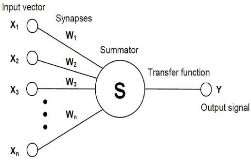
From a computational point of view, NN is a structure that includes itself a certain number of processing elements that execute a fixed set of mathematical functions. This processing element is called an artificial neuron (AN). It consists of an input vector (X_i), synapses, a summation, a nonlinear transfer function and an output signal value (Figure 1) [5-7].

Figure 1: A scheme of an elementary processor (AN).

AN executes the following operations:

$S={\displaystyle \sum _{i=1}^n{X}_i{W}_i};Y=f\left(S\right);f(S)=\frac{1}{1+e^{-\alpha S}}$

The task of synapses is to multiply the input vector components X_i by a number characterizing the synapse strength (it is called synaptic weight W_i). These values obtained are summed and the sum is fed to the transfer function Y whose role is played by a monotonous function of one argument (usually sigmoid function f(S)). Thus, AN maps the vector X_i to a scalar value Y.

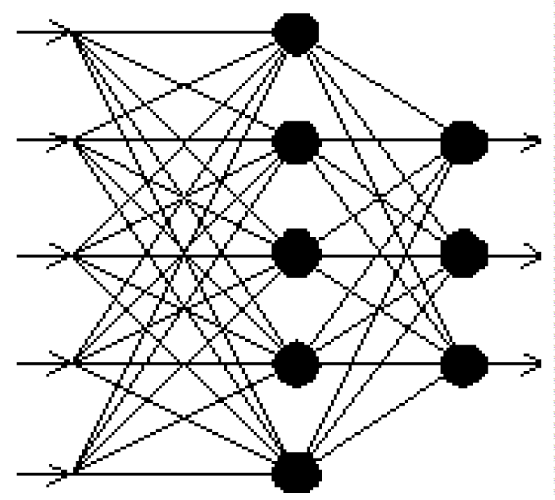
The number of “neurons” and the scheme of connection of them with each other can vary. NN can be presented often as “neurons” formed in layers. The “neurons” in a layer are not connected with each other, but they are connected with neurons of the previous and next layers by the principle “each with each.” The simplest kind of NN is feed-forward NN, whose ANs are grouped into layers – Figure 2. [5]

Figure 2: A scheme of NN that consists of one input layer, one “hidden” layer, and one output layer.

The NN in Figure 2 consists of one input nodes layer (5 input nodes), one hidden layer (5 AN), and one output layer (3 AN). Input nodes serve just as signal sources while all the other AN perform the computations described above.

This computational structure can approximate dependencies between input variables and target (output) variables (functions) of an object after training on a set of experimental data.

The essence of training is selecting the correct synaptic weights.

In the process of training, the weights of all synapses are determined from the requirement that NN should map all known input vectors to the known corresponding values of the target variables with minimum error.

This process is organized as follows. The initial synaptic weights are set using a random number generator. Then, a random input vector of real data is selected and fed to the NN. The NN calculates an output value, it is compared with the expected output value and the respective error is calculated. Using the “error backpropagation” algorithm based on the classic gradient descent method [8-10], synaptic weights are changed by certain values. After that, a new input vector of real data is randomly selected and the whole weight update procedure is repeated. The procedure is repeated until an acceptable difference between the values computed by NN and the real values of the target variable is reached.

The number of training cycles can be more than 500-1000.

The resulting NN is able to true to map any input vector close to the vectors used during training into the respective value of the target variable i.e. to approximate the dependence of a target variable on input factors.

Applications of neural networks. Rules, tips, examples

The organization of real data to be used for NN training is very important.

The data for NN training (consisting of input variable value vectors and output values corresponding to them) can be formed by means of various techniques. They can contain data measured in real experiments or data obtained from numerical simulations; they can contain data of both types when these data can complement each other.

The data must be cleared, that is, contradictions, duplicates, and anomalous values must be excluded.

The data should be evenly distributed over the area of the input vector space, it is necessary to avoid large differences in data density in different parts of this area.

The data should be supplemented with metadata containing additional information about the object, for example, physical or chemical constants characterizing the object under study, the parameters of the technology for creating the object, etc. [11-13].

The use of metadata as additional data not only increases the accuracy of the NN model but also allows a deeper understanding of the physicochemical nature of the objects of research and the fine details of the mechanism of the processes under study.

Another significant circumstance is the proper choice of NN structure for which certain theoretical and empirical rules exist.

For example, one of the general rules (confirmed by our experience [5,7,11-13]) is that number of synapses should be 3 - 5 times less than the number of input vectors (examples) used in training. The use of NN with a greater number of synapses may lead to the so call over-fitting.

The loss of the ability to generalize means that the NN remembers training examples well and accurately reproduces the target variables for the training input vectors, but gives erroneous values of the target variables for the input vectors that we did not use in training.

To find out if the NN has the ability to generalize the dependencies contained in the data, the following approach is used. In the process of training, the input vectors (a set of examples) are divided into two groups. A large group is used for training, and a smaller group is used only to check the NN prediction accuracy. If the NN accuracy in both groups is approximately the same, the NN is not retrained and has the ability to identify and generalize the dependencies of existing data.

One more rule: it has been empirically established that it is better to use three separate NN for each of the three “outputs” than one NN for all “outputs” (Figure 2).

The general principle for NN structure selection is as follows. For the majority of tasks, 2 hidden NN layers are sufficient to obtain an acceptable error level. Therefore, using NN with more than 2 hidden layers can hardly make sense in many cases. Moreover, the accuracy of networks with a single hidden layer (Figure 2) is often quite good for problems of physics and natural science where dependencies are deterministic.

The final choice of the optimal NN structure for each research task is carried out empirically - by checking the exactness of different NN (for example, with a different number of AN in the hidden layer).

It should be noted here that all questions of the methodology of NN used for approximating experimental data have been well worked out both from a theoretical and practical point of view at present. There exist a number of academic (free) and professional software packages which support all steps of data pre-processing, NN training, model results visualization, model quality evaluation and validation as well as make modeling experimental data simple and convenient.

Therefore, at present, it is possible to put forward the motto that experimental work cannot be considered complete until the MCM of experimental data has been created.

We believe that an autonomous executable module of the NN model created by the authors of the article should be a mandatory supplement to any scientific article. This is explained as follows. A correctly created NN model is, first of all, the most complete form of presentation of experimental results, since the NN model contains the relationships between all the variables of the experiment.

This will allow any reader of the article, having received the autonomous executable module, independently examine in detail all the regularities contained in the NN model, visualize in the form of graphs those regularities that the authors of the article could not cite in the article due to limitations on the volume of the article.

An additional advantage of the autonomous executable module of the NN model is that, with its help, the reader of the article can conduct “virtual experiments” [14-17], setting such combinations of factor values that were not investigated in the published article.

The virtual experiments can also be carried out to extrapolate dependencies revealed by the NN model (that is, to solve forecasting problems).

The virtual experiments can also be carried out to execute unique experiments for such combinations of factor values that cannot be organized or are difficult to organize.

In addition to the above, one more, very interesting, the case should be noted when the use of NN is justified. Our experience shows that the Root-Mean-Square (RMS) error of the NN model is always less than the RMS error of the experimental data used to create the NN model. This allows the NN model to be used as a means of checking the quality of the experiment as a whole! Moreover, both from the point of view of the measurement error of the variables of the experiment and from the point of view of the correctness of the experiment, that is, the completeness of taking into account all the factors affecting the objective function of the experiment.

In cases where the RMS error of the NN model is too large (for example, when the RMS error of the NN model is more than 10-3), it is necessary to improve the accuracy of the experimental variables measurement and (or) change the formulation of the experimental problem, trying to take into account additional factors affecting the objective function of the experiment.

A series of more specific rules and various examples of real research results on the combustion and detonation of high-energy materials are presented in the easily accessible works by the authors [13-17].

Conclusion

The use of neural networks for approximating experimental data is a well-established methodology with both theoretical and practical foundations. The quality of the data used for training is crucial, and it should be cleared of contradictions, duplicates and anomalous values. Metadata containing additional information about the object under study should also be included to increase the accuracy of the model and allow a deeper understanding of the processes involved. The choice of the optimal neural network structure should be carried out empirically, and certain rules should be followed, such as using three separate neural networks for each output and limiting the number of hidden layers to two. With the availability of academic and professional software packages, creating a model for experimental data has become simple and convenient, and it can be argued that experimental work cannot be considered complete until a neural network model has been created.

1. Kolmogorov A. On the representation of continuous functions of several variables by superpositions of continuous functions of a smaller number of variables. Izvestiya AN SSSR. 1956; 108:179-182.
2. Arnold V. On the function of three variables. Izvestiya AN SSSR. 1957; 114(4):679-681.
3. Gorban AN. Generalized approximation theorem and computational capabilities of neural networks. Siberian Journal of Computational Mathematics. 1998; 1(1):11-24.
4. Hecht-Nielsen R. Kolmogorov's Mapping Neural Network Existence Theorem. IEEE First Annual Int. Conf. on Neural Networks, San Diego. 1987; 3:11-13.
5. Abrukov VS, Karlovich EV, Afanasyev VN, Semenov YV, Abrukov SV. Creation of propellant combustion models by means of data mining tools. International Journal of Energetic Materials and Chemical Propulsion. 2010; 9(5):385-394.
6. Chandrasekaran N, Oommen C, Kumar VRS, Lukin AN, Abrukov VS, Anufrieva DA. Prediction of Detonation Velocity and N − O Composition of High Energy C − H − N − O Explosives by Means of Artificial Neural Networks. J. Propellants, Explosives, Pyrotechnics. 2019; 44(5):579-587.
7. Abrukov VS, Lukin AN, Oommen C, Chandrasekaran N, Bharath RS, Kumar VRS, Anufrieva DA. Development of the Multifactorial Computational Models of the Solid Propellants Combustion by Means of Data Science Methods - Phase II. Technology and Investment, Proceedings of a meeting held 9-11 July 2018, Cincinnati, Ohio, USA. Held at the AIAA Propulsion and Energy Forum. 2018; AIAA 2018-4961.
8. Werbos PJ. Beyond regression: New tools for prediction and analysis in the behavioral sciences (Doctoral dissertation). Harvard University, Cambridge, MA. 1974.
9. Galushkin AI. Synthesis of multilayer image recognition systems. M.: Energy. 1974.
10. Rumelhart DE, Hinton GE, Williams RJ. Learning Internal Representations by Error Propagation. In: Parallel Distributed Processing. Cambridge. 1986; 1:318-362.
11. Abrukov VS, Kochergin AV, Anufrieva DA. Artificial neural networks as a means of generalizing experimental data. Bulletin of the Chuvash University. 2016; 3:155-162. https://www.researchgate.net/publication/333211155_Iskusstvennye_nejronnye_seti_kak_sredstvo_obobsenia_eksperimentalnyh_dannyh_artificial_neural_networalks_as_fa_meata.
12. Anufrieva DA, Koshcheev MI, Abrukov VS. Application of data mining methods in physics research. Multifactor detonation models. In the collection: High-speed hydrodynamics and shipbuilding. Collection of scientific papers of the XII International Summer Scientific School-Conference dedicated to the 155th anniversary of the birth of Academician A.N. Krylov. 2018; 221-226. https://www.researchgate.net/publication/333210244_Primenenie_metodov_intellektualnogo_analiza_dannyh_v_fiziceskih_issledovaniah_mnogofaktornye_modeli_detonacii .
13. Anufrieva DA, Abrukov VS, Lukin AN, Oommen C, Sanalkumar VR, Chandrasekaran N. Generalized multifactor computational models of the detonation of condensed and gas systems. 2019. https://www.researchgate.net/publication/334126580_Generalized_multifactor_computational_models_of_the_detonation_of_condensed_systems
14. Abrukov VS, Anufrieva DA, Sanalkumar VR, Mariappan A. Multifactor Computational Models of the Effect of Catalysts on the Combustion of Ballistic Powders (experimental results of Denisyuk team) Direct Tasks, Virtual Experiments and Inverse Problems. 2020. https://www.researchgate.net/publication/344727996_Multifactor_Computational_Models_of_the_Effect_of_Catalysts_on_the_Combustion_of_Ballistic_Powders_experimental_results_of_Denisyuk_team_Direct_Tasks_Virtual_Experiments_and_Inverse_Problems
15. Abrukov VS, Anufrieva DA, Sanalkumar VR, Mariappan A. Comprehensive study of AP particle size and concentration effects on the burning rate of composite AP / HTPB propellants by means of neural networks: Development of the multifactor computational models. Direct tasks and inverse problems & virtual experiments. 2020; 1-20. https://doi.org/10.13140/RG.2.2.19019.62242
16. Abrukov V, Anufrieva DA, Lukin AN, Oommen C, Sanalkumar VR, Chandrasekaran N. Effects of metals and termites adds on combustion of double-based solid propellants: Development of the multifactor computational models of the solid propellants combustion by means of data science methods. Virtual experiments and propellant combustion genome. 2019. https://www.researchgate.net/publication/334172872_Effects_of_metals_and_termites_adds_on_combustion_of_double-_based_solid_propellants_development_of_the_multifactor_computational_models_of_the_solid_propellants_combustion_by_means_of_data_science_me
17. Pang W, Abrukov V, Anufrieva D, Chen D. Burning rate prediction of solid rocket propellant (SRP) with high-energy materials genome (HEMG). Crystals. 2023; 13(5):237. doi: 10.3390/cryst13050237.