Comparative analysis of speech coders

In this paper a comparative analysis of some of the most popular speech coders is presented. Qualitatively and quantitatively are tested Linear Prediction Coding in its implementation LPC-10e and with the use of auto-correlation and covariance, companding coding including A-law and µ-Law, ADPCM IMA, G.726 A- and µ-Law, and a fully featured MELP coder. All of them proved their efficiency for the typical applications they have been assign to providing the necessary quality vs. output data rate. The methodology for evaluation along with the codecs’ descriptions are considered useful for new coming specialists in the field of audio compression as one possible starting point for them.

Introduction

In this paper is presented a comparative analysis of four speech codecs – Linear Predictive Coding (LPC), Companding (A-law and μ-law), Adaptive Pulse Code Modulation (ADPC), and Mixed Excitation Linear Prediction (MELP). Representing some of the basic steps of speech processing with the ultimate goal of achieving as higher as possible compression ratio, while retaining tolerable good quality of the voice, they are highly popular in modern telecommunications. Thus, a great interest is posed to them during the university studies of students into the courses on Audio Technologies. In [1], according to Chu, are classified some of the main properties defining the audio quality as a subjective estimate for recorded speech – intelligibility, naturalness (pleasantness), and speaker recognisability. They depend on several of factors such as dependency on speaker, language, signal levels, background noise, tandem coding, channel errors, presence of non-speech signals which need to be considered altogether. The main goal of this evaluation is to present, mainly to newly arising specialists, a systematic approach for estimation of key parameters that demonstrate the qualities of the considered algorithms along with their basic description.

Part II of this publication consists of general depiction of each of the tested codecs, followed by a comparative test results in Part III which are then discussed in Part IV and a brief conclusion is given in Part V.

Codecs description

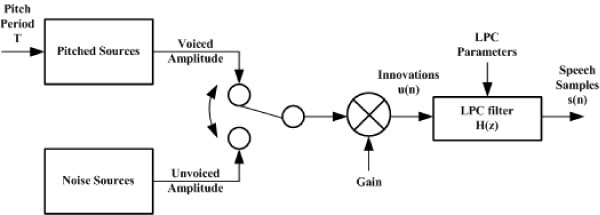
The general concept of the Linear Predictive Coding (LPC) [2] is presented in Figure 1. It is a basic way for representing a speech signal in shorter form. It is embedded as a key processing step in many more complex contemporary speech codecs. Typically, speech is taken from the input in short segments. One of the underlying characteristics for them is the shape of the spectrum. Having a small number of parameters which describe it could be used for compacting. Since, a single speech sample is considered correlated to previous ones in time, it can be derived nearly by combining them linearly.

Figure 1: LPC coder, as described in [2].

The output samples sp(n) of the speech are obtained from the sum of previous samples s which are weighted:

$s_p(n)={\displaystyle \sum _{i=1}^{p}a(i)s(n-i)}\text{ (1)}$

which inevitably leads to an error e(n):

$e(n)=s(n)-s_p(n)=s(n)-{\displaystyle \sum _{i=1}^{p}a(i)s(n-i)}\text{ (2)}$

All a(i) could be estimated by finding the minimum of the cumulative squared error E for the whole segment:

$E={\displaystyle \sum _n{e}^2(n)}\text{ (3)}$

Actually, the speech samples s(n)are generated under the influence of excitation signal u(n) with the following relation:

$s(n)={\displaystyle \sum _{i=1}^{p}a(i)s(n)}+u(n)\text{ (4)}$

In this process a LPC filter is applied with the following transfer function:

$H(z)=\frac{1}{A(z)},A(z)=1-{\displaystyle \sum _{i=1}^{p}a(i)z^{-i}}\text{ (5)}$

being fed by a noise (white) source and a voiced source with a pitch period T.

Talking about the Public Switched Telephone Network (PSTN) the well adapted and most often used speech codecs are the A-law and μ-law. The amplitudes of the input voice samples are being transferred by using a logarithm type function, actually achieving nonlinear quantization. The reason for employing a nonlinear transformation instead of a linear one is the nature of speech levels distribution. Most often the mid-range amplitudes are met in contrast to small and very large ones which the human ear perceives better. Companding (compressing and expanding) the user’s signal comes to as a natural solution – levels not affecting human speech perception are suppressed and the rest – kept as close to the original as possible. Then uniform quantization is applied. At reception point dequantization is implemented followed by expansion. United States and Japan use μ-law in their systems while A-law is employed in the other countries around the world and both come into the G.711 standard of ITU [3].

Transformation of the input signal s after initial normalization within the range of [-1, +1] following μ-law in 8-bit values is done according to:

$f(s)=\frac{\ln (1+\mu \left|s\right|)}{\ln (1+\mu )}\mathrm{sgn}(s)\text{ (6)}$

where μ is positive integer (companding factor). The recommended value for it is 255.

The 8-bit A-law variation is represented by:

$f(s)=\{\begin{array}{c}\frac{A\left|s\right|}{1+\ln (A)},0\le \left|x\right|\le \frac{1}{A}\\ \frac{1+\ln (A\left|s\right|)}{1+\ln (A)},\frac{1}{A}\le \left|s\right|\le 1\end{array}\text{ (7)}$

where A is recommended to be 87.6.

ADPCM is a sequel of the differential pulse code modulation. At it there is preserving only of the differences between samples while the size of the quantization step is changing for achieving higher compression ratios at given signal-to-noise ratio (SNR). Differences for adjacent samples tend to be very small frequently due to the considerable correlation of a voice signal in a small time period and they could be represented with less number of bits. Here a prediction is also applied of the speech signal and then the difference is calculated with it. Lower errors indicate more accurate prediction and in the general case it leads to lower dynamic range for he transmitted signal. Quantization, then, can be done with a fewer bits instead of using the original scale for input samples. The main processing steps of the algorithm are shown in Figure 2.

Figure 2: ADPCM codec, as described in [4].

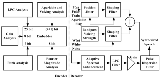
PCM values between the input sample x(n) and the predicted one derived from the previous xP(n-1) are calculated. While decoding, the quantized difference signal is put together with the predicted to regenerate the speech signal. Adaptive prediction and quantization improve the overall performance of the codec considering the variation in the speech signal. The quantizer is changing the step size conforming to the wave shape under processing. There are different implementations of the ADPCM algorithm. One of the most popular is described in G.726 [4] recommended by the Interactive Multimedia Association (IMA) and the International Telecommunication Union (ITU). Here, linear PCM samples are placed into 4-bit values after the quantization starting from 16-bit per sample out from 8 kHz single channel. Initially, 128 kbps capacity per link is required which after compression falls down to 32 kbps. Operation is foreseen, also, at 40, 32, 24 and 16 kbps due to the adaptive speed control. The hard switching between voiced and unvoiced segments, pledged in LPC based voice coders, is considerable disadvantage producing errors when fricatives are processed. It can be solved by the introduction of second decision module about the current voice segment using multiple frequency bands. Mixed Excitation Linear Prediction (MELP) is such a solution. Short-term spectrum is analysed by LPC analysis eliminating the binary decision for voiced vs. unvoiced presence characterizing the full segments. Excitation is modelled by estimation of periodic and noise-like components rendering an account of their weight on forming the voice strength over different bands in spectrum domain. Four new features are introduced, apart from the LPC parameters – mixed pulse, noise excitation, aperiodic pulses, pulse dispersion and adaptive spectral enhancement.

Periodic and aperiodic pulses are included during the speech synthesis when the current frame consists of voice samples in the case of MELP. Aperiodic ones help in reducing distortions from the LPC module signal generation which happens for isolated sounds. They are typical for transitional regions where voice is followed by non-voice segments and vice versa. Figure 3 depicts the structure of the MELP codec.

Figure 3: MELP codec, as described in [5].

Differences between untouched and synthesised voice where no formant is present are diminished by the pulse dispersion filter assuring slower collapse between pitch peaks. Excitation energy is more evenly distributed considering the period of the latter for better quality.

Post-filtering is also provided for adaptive spectral enhancement. LPC residual part could be represented by Fourier coefficients leading to complemented presentation of the excitation signal. Thus, the spectral shape is included for processing helping for better reproduction of lower frequencies in contrast to the LPC.

Experimental results

The input non-compressed audio of a female speech is contained in wav-format file representing mono signal with a sample rate of 8 kHz and 16 bits/sample. Its length is 20 sec. For the evaluation of the codecs described in Section II the following quantitative parameters are used [6]:

Signal-to-Noise Ratio (SNR):

$SNR=10{\log }_{10}\frac{{\displaystyle \sum _{n=o}^{N-1}{s}^2(n)}}{{\displaystyle \sum _{n=0}^{N-1}{[s(n)-\stackrel{⌢}{s}(n)]}^2}},dB\text{ (8)}$

where s and $\stackrel{⌢}{s}$ are the original and restored speech signals, respectively; N – the total number of samples processed;

Log Spectral Distance (LSD):

$LSD=\frac{1}{L}{\displaystyle \sum _{l=0}^{L-1}\sqrt{\left\{\frac{1}{K/2+1}{\displaystyle \sum _{k=0}^{K/2}\left[10{\log }_{10}{\left|t(k,l)\right|}^2-10{\log }_{10}{\left|\stackrel{⌢}{t}(k,l)\right|}^2\right]}\right\}}},dB\text{ (9)}$

where L is the number of processed segments; K – their length in number of samples; t and $\stackrel{⌢}{t}$ are the spectral powers of a segment prior to and after processing. The Perceptual Evaluation of Speech Quality Mean Opinion Score (PESQMOS) is found according to the ITU-T recommendation P.862 [7] (Table 1).

Discussion

The audible evaluation of the resulting samples shows that there is a little hissing around the consonants in for the LPC-10e coder. Some mid consonants in between vocals seem shortened which gives a bit computerized sounding when autocorrelation method is switched on in LPC. There is detectable nasal hue at the end of vocals preceding pauses which also give prolonged sounding. The companding approach using both A-law and µ-Law assures very clear distinction between vocals and consonants with just a little bit hiss addition in steepest transitions for µ-Law. ADPCM codec variants are very close in results of subject appraisal to companding with hardly discoverable for the A-law a little noised prolongation at the end of some words where vocals reside. Emphasized consonants appear in the speech processed by MELP in all parts with lower level of persistent noise (as background presence) and with no buzziness effects.

Conclusion

The quantitative and qualitative evaluation of the LPC, Companding, ADPCM, and MELP speech coders are with mutual agreement proving them as applicable within systems providing voice services of mass type. There could be noted some significant improvement of the quality based on both SNR and PESQMOS measures for the group of Companding and ADPCM algorithms regardless of the type of transformation inside, whether it is A-law or µ-Law. All quality variations are compensated by the achieved data rates proper for the respective applications.

1. Chu WC (2003) Speech Coding Algorithms: Foundation and Evolution of Standardized Coders, New Jersey, USA: John Wiley & Sons. Link: https://bit.ly/2xtX74M
2. Makhoul J (1975) Linear prediction: A tutorial review, Proceedings of the IEEE. 63: 561-580. Link: https://bit.ly/3aoZ8Os
3. G.711 (1988) Pulse code modulation (PCM) of voice frequencies, ITU-T Recommendation (11/1988), Link: https://bit.ly/2JlIALb
4. Salomon D (2007) Data Compression, The Complete Reference, 4 ed., London, UK, Springer. Link: https://bit.ly/2ya2WF6
5. Supplee L, Cohn R, ColluraJ, McCree A (1997) MELP: The new federal standard at 2400 bps”, In Proc. of the 1997 IEEE International Conference on Acoustics, Speech, and Signal Processing (ICASSP-97), Münich, Germany 1591-1594. Link: https://bit.ly/2JcOe2r
6. Benesty J, Makino S, Chen J (2005) Speech Enhancement, Springer. Link: https://bit.ly/2QGBdCn
7. ITU-T Recommendation P.862 (2001) Perceptual evaluation of speech quality (PESQ): An objective method for end-to-end speech quality assessment of narrow-band telephone networks and speech codecs. Link: https://bit.ly/2vPHXGR