A model predictive approach to control vehicle skidding by sideslip angle estimation

Nowadays, many cars are equipped with Advanced Driving Assistance Systems (ADAS), from cruise control to collision detection and speed limit signalling. In recent years, the scientific community has carried out a lot of research in the field of autonomous driving system with the aim of improving fuel consumption, traffic and safety, but it is still a developing field that will require a lot of work despite the great progress. This paper proposes a new approach to road safety, introducing an autonomous driving system that intervenes when dangerous situations occur or when the driver is not able to drive, keeping the passengers and the other vehicles safe.

A Linear Time Varying (LTV) Model Predictive Control (MPC) is proposed to control the vehicle minimising the lateral error with respect to lane centre while maintaining a constant speed. The lane centre is estimated by the lane boundaries that are supposed to be given by a vision detection system.

The risk situation is evaluated by the slip angle and rate.

Introduction

Road safety is an important issue in these years. The number of deaths on roadways are 1.35 million around the world each year [1] and the main reason of an accident could depend of the actions of the driver [2]. Recently manufactured cars are investing in research to create autonomous system able to prevent and avoid risky situations. One of these dangerous conditions regards a context in which the driver loses the control of the car: sliding or braking sharply by external and unexpected events. Different systems may detect these anomalous states: some using the human like a sensor by EEG signal [3] or biometric t-shirt [4]. Recent research advancements in technology focuses on active safety technology (AST) regarding the ADAS that assists drivers in driving. In [5] is shown how this technology can reduce the number of crashes by considering different possible traffic situations. Another positive aspect regards the reduction of fuel consuption and traffic congestions through vehicle control optimization and platooning [6].

In this context, it is important to provide alternative systems able to detect the risky situation and improve the safety on road. The focus of the control system proposed in this paper is to improve the technology of the ADAS.

In this paper, the proposed system does not consider only a specific speed or a position for the car which covers a straight lane, but its focuses on the detection of the risk situations through the data coming from the automotive system as the slip angle. According to the acquired data, the model takes the full control of the car in order to recover from errors due to human operator and restore a safe state. In these cases, a process able to increase the autonomy level in the human-machine system is fundamental [7]. Another positive aspect is the resilience of the system to the external events [8]. The slip angle is extremely useful in many safety application [9] to prevent some risk situation. The slip angle can be estimated using the steering torque [10] or using the wheel speed and lateral acceleration [11]. Those latter automotive data is evaluated by sensors located in the car in order to shift toward a state of autonomous system in order to take the control and react without human intervention. In this paper the slip value is evaluated by a Kalman Filter that estimates the lateral speed of the chassis and computes the sideslip angle.

Methods and materials

Vehicle model

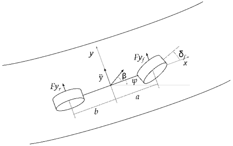
The linear yaw-plane bicycle model (Figure 1) is adopted to design the Model Predictive Control and it is used to make predictions on the states of the vehicle.

Where:

• y is the lateral displacement;

• is the lateral speed;

• is the yaw angle;

• is the yaw rate;

• δ is the steering angle of the front wheels while it is assumed that the rear wheel is not able to turn;

• and are the lateral forces generated by the wheel

• a is the distance from the front axis and the Centre of Gravity (CG);

• b is distance from the rear axis and the CG;

The adopted model considers a linear tyre model where the wheels dynamics are linearized with a constant stiffness coefficient Cf for the front wheel, Cr for the rear wheel) as shown in Figure 2.

Thus, the forces and are defined as follows:

$F_{y_f}=2C_f{\alpha }_f$ $F_{y_r}=2C_r{\alpha }_r$ (1)

Where αf and αr are the drift angle of the front and rear wheel, defined as:

${\alpha }_f={\delta }_f-\frac{\dot{y}-\text{a}\dot{\psi }}{\dot{x}}$ ${\alpha }_r={\delta }_r-\frac{\dot{y}-\text{b}\dot{\psi }}{\dot{x}}$ (2)

The linearization of the wheel model implies a less accurate computation of the lateral and longitudinal force generated by the wheel while driving and breaking; however, since the goal of the system is to keep the vehicle in the linear region of the wheels dynamics it is possible to use this approximation. Further improvements of the system include the implementation of better models such as the Magic Formula.

Thus, the continuous state space representation is defined as follows:

$\dot{X}=AX+Bu$ (3)

Where $X={\left[\begin{array}{cccc}y& \dot{y}& \psi & \dot{\psi }\end{array}\right]}^T$ is the state vector and u = δ is the control input.

The state space matrices A and B are defined as follows:

$A=\left[\begin{array}{cccc}0& 1& 0& 0\\ 0& -\frac{2\left(C_f+C_r\right)}{m\dot{x}}& 0& -\dot{x}-\frac{2\left(a{C}_f-b{C}_r\right)}{m\dot{x}}\\ 0& 0& 0& 1\\ 0& -\frac{2\left(C_f+C_r\right)}{I_{zz}\dot{x}}& 0& -\frac{2\left(a^2{C}_f+b{C}_r\right)}{I_{zz}\dot{x}}\end{array}\right]$ $B=\left[\begin{array}{c}0\\ \frac{2C_f}{m}\\ 0\\ \frac{2a{C}_f}{I_{zz}}\end{array}\right]$ $C=\left[\begin{array}{cccc}1& 0& 0& 0\\ 0& 0& 1& 0\end{array}\right]$ (4)

Then the proposed model is discretized by Euler Method:

$A_k=A*Ts+I_{n\times n}$ $B_k=B*Ts$ $C_k=C$ (5)

Where:

$C_k=C$ is the longitudinal speed of the vehicle;

$C_{f,r}$ is the stiffness coefficient of the front (f) and rear (r) tyre;

m is the mass of the vehicle;

$I_{zz}$ is the inertia on the z-axis.

Ts is the sampling time.

Activation criteria

The proposed autonomous system has to be activated when specific conditions that could lead to dangerous situations occur, such as oversteering or understeering.

The sideslip angle is a significant parameter in the detection of the risk due to situations where the vehicle starts to lose control. Thus, the analysis of the sideslip angle value allows to prevent the loss of control and it provides efficient information to effectively apply an ad-hoc control law. The slip angle can be obtained using the relationship in (6):

$\beta =\arctan \left(\frac{\dot{y}}{\dot{x}}\right)$ (6)

Where β is the sideslip angle, and are respectively the lateral speed and longitudinal speed of the CG of the vehicle.

In the proposed approach, the data coming from the sensor (accelerometer) which stores the longitudinal and lateral acceleration and yaw rate is affected by white noises due to measurement errors. In order to provide an optimal filtering of such noises in the measurements and to generate a good estimator for the sideslip angle β, a Kalman Filter (KF) is adopted. Thus, the criteria will be:

$\left|\widehat{\beta }\right|\le {\beta }_{lim}$ $\left|\widehat{\dot{\beta }}\right|\le {\dot{\beta }}_{lim}$ (7)

Where β and are respectively the estimated sideslip angle and rate while and are the related threshold limit values over which the controller starts.

The KF, instead of using the model proposed in (4), is based is based only on the dynamic equation of lateral speed and yaw rate , and only the lateral speed is supposed to be measurable from the accelerometer:

$\Omega =\left[\begin{array}{cc}-\frac{2\left(C_f+C_r\right)}{m\dot{x}}& -\dot{x}-\frac{2\left(a{C}_f-b{C}_r\right)}{m\dot{x}}\\ -\frac{2\left(C_f+C_r\right)}{I_{zz}\dot{x}}& -\frac{2\left(a^2{C}_f+b{C}_r\right)}{I_{zz}\dot{x}}\end{array}\right]$ $\Psi =\left[\begin{array}{c}\frac{2C_f}{m}\\ \frac{2a{C}_f}{I_{zz}}\end{array}\right]$ (8) ${\rm H}=\left[\begin{array}{cc}1& 0\end{array}\right]$

The model is linearised and discretised around the operating point which represents the current vehicle speed. Due to the presence of noises on state measurements, the state space representation may be formalized as follows:

${\eta }_{k+1}={\Omega }_k{\eta }_k+{\Psi }_k{U}_k+w_k$ ${\Phi }_k={{\rm H}}_{\text{k}}{\eta }_{\text{k}}$ (9)

Where:

${\eta }_k=\left[\begin{array}{cc}{\dot{y}}_k& {\dot{\psi }}_k\end{array}\right]$

${\Omega }_k$ , ${\Psi }_k$ and ${{\rm H}}_k$ are the discretised matrices with Euler method as in (5)

$w_k$ is the noise on the state at time k

The KF implements the following recursive equations:

1. Prediction phase

${\tilde{\eta }}_k={\Omega }_k{\eta }_k+{\Psi }_k{U}_k+w_k$ (10)

2. Update of error covariance matrix P and Kalman gain K

$P={\Omega }^{\text{T}}P\Omega +\text{Q}$ $K=P{{\rm H}}^T\left({\rm H}P{{\rm H}}^T+R\right)$ (11)

3. Update the state estimation

${\tilde{\eta }}_k={\tilde{\eta }}_k+K\left(y_{measurements}-{\rm H}{\tilde{\eta }}_k\right)$ (12)

4. Update of error covariance matrix P

$P=\left(I-K{\rm H}\right)P{\left(I-K{\rm H}\right)}^T+KR{K}^T$ (13)

For each time interval, the KF estimates the state of the system, and the sideslip angle is computed by the equation (6).

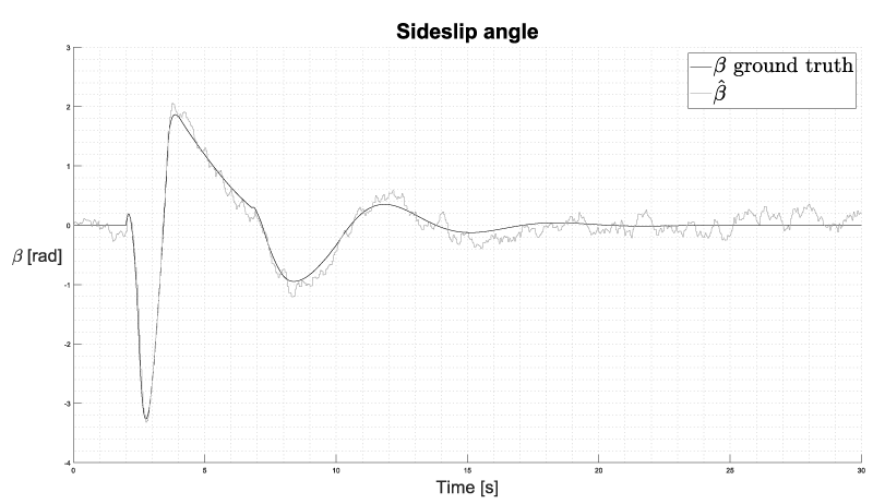
In Figure 3 is shown the result of the estimation process during the simulation. The KF correctly estimates the sideslip angle with a maximum error of 0.011 and an average error of -1.5∙10-4 with respect to the ground truth which is given by the simulation software.

Lane keeping control

When the sideslip angle overcomes the thresholds, the vehicle control, consisting in a Lane Keeping System, starts and keeps the vehicle control.

The control system is based on the dynamic Linear Time Varying System (LTV) model proposed in (4). According to [12], in fact, the dynamic model performs a robust estimate in respect to the kinematic model which is fast and simple to be applied but it is very sensitive to noise on measurements, above all for the accelerations measurements which are affected by high errors. For these reasons, in this kind of application, the use of a dynamic model is recommended.

The aim of the proposed control law is to minimize the quadratic cost function J to converge the lateral offset to zero.

It is supposed to have the lane boundaries from a camera located on the front of the vehicle using a vision detection algorithm. In respect to the boundaries, the lateral offsets with respect to the vehicle, the centre of the lane and the respective lateral offset are computed. The simulation software gives data subjected to measurements error/noise. More noise is in the data, less precise would be the controller response in terms of oscillations with respect to the centre of the lane. In this case of study, the simulated sensor has a measurement error of 3 centimetres. In order to improve the performance of the system, an accurate tuning of the KF is required to filter the noises of the sensors.

To improve the controller performances, the following formulation of the augmented state for the model presented in (6) is derived

$State: \left[\begin{array}{c}y\\ \dot{y}\\ \psi \\ \dot{\psi }\end{array}\right]\to \left[\begin{array}{c}y\\ \dot{y}\\ \psi \\ \dot{\psi }\\ \delta \end{array}\right], input: \left[\delta \right]\to \left[\Delta \delta \right]$ (14)

Consequentially, with an abuse of notation, the model matrices are redefined as follows:

$A_k=\left[\begin{array}{cc}{A}_k& B_k\\ 0& I\end{array}\right], B_k=\left[\begin{array}{c}{B}_k\\ I\end{array}\right], C_k=\left[\begin{array}{cc}{C}_k& 0\end{array}\right]$ (15)

Thus, the cost function is defined as follow and it is minimized at each time step over a prediction horizon Np:

$J={\left(Y_{r,N}-C{X}_N\right)}^T{Q}_N\left(Y_{r,N}-C{X}_N\right)+{\displaystyle \sum }_{k=0}^{N-1}\left[{\left(Y_{r,k}-C{X}_k\right)}^{T}Q\left(Y_{r,k}-C{X}_k\right)+\text{Δ}{U}_k^{T}R\text{Δ}{U}_k\right]$ (16)

Where:

$Y_{r,k}$ is the reference at time k;

$X_k$ is the vehicle state at time k;

$U_k$ is the optimization vector consisting in the steering angle;

The matrices QN, Q and R are optimization matrices tuned by hand.

The minimization problem is subjected to specific constraints to achieve better results. The constraints are applied on the control variables and their rate in time over the control horizon Nc.

Some considerations must be made on the upper and lower bound for the control Uk. The objective of the control system is to avoid high values for the sideslip angle which may produce over or under steering situations with the consequent losing control of the vehicle. So, inappropriate setting of the bound values may induce the MPC to react too strongly generating a high value of counter steer resulting in a drift. To avoid such behaviour, a dynamic constraint is applied to the steering wheel.

The approach proposed in this paper approximates the longitudinal acceleration to zero since the rate of change of the speed over the prediction horizon could be negligible. As shown in [14], the lateral acceleration of the vehicle must be bounded by the tyre-road friction coefficient, thus resulting in the following relation:

$\left|a_y\right|\le \mu g$ (17)

Where ay is the lateral acceleration, µ is the road friction and g is the gravity force.

The lateral acceleration could also be expressed in function of the curvature of the vehicle trajectory:

$a_y\approx {\dot{x}}_0^2*{\kappa }_k$ ${\kappa }_k=\frac{1}{R_k}, R_k=\frac{L}{2\sin {\delta }_k}$ (18)

where kk is the curvature at time k, Rk is the turning radius of a vehicle with the steering angle at time and wheelbase L. The steering angle is then derived from equations (18) and (17):

$\varphi =\{\begin{array}{c}\frac{L\mu g}{2{\dot{x}}_0^2}, if \left|\varphi \right|\le 1\\ -1, if \varphi \le -1\\ 1, if \varphi \ge 1\end{array}$ (19a)

${\delta }_k=asin\left(\varphi \right)$ (19b)

The argument of the arcsine function (19b) is limited between [-1,1] (19a) and the result is capped to physical limits of the steering system.

Thus, the δ computation became:

$\{\begin{array}{c}{\delta }_{ub}={\delta }_{lim,ub}, if \left|{\delta }_{lim,ub}\right|\ge {\delta }_{physical,ub}\\ {\delta }_{lb}={\delta }_{lim,lb}, if \left|{\delta }_{lim,lb}\right|\le {\delta }_{physical,lb}\end{array}$ (20)

Where is the limit obtained by equation (20) and is the physical limit of the steering system.

The limit of a steering system depends on different characteristics such as physical space available for wheels and steering linkage geometry (Ackermann, Anti-Ackerman, Bell-crank, Rack-and-Pinion, Short Rack-and-Pinion). The proposed system uses a limit that should be feasible for the most types of cars.

The resulting is used as constraint for current time instant over the control horizon. In Figure 4 are shown the different limits of in respect to the longitudinal speed of the vehicle on a high adhesion (µ = 0.8). Thus, the complete optimization problem became:

$\Delta {\delta }^{*}=\underset{\Delta {\delta }^{*}}{\min }J\left(X,\Delta \delta \right)$ $X_{k+1}=A_k{X}_k+B_k\Delta {\delta }_k, k=0,\dots ,N_p$ $Y_k=C_k{X}_k, k=0,\dots ,N_p$ ${\delta }_{lb}\le \Delta {\delta }_k+{\delta }_{k-1}\le {\delta }_{ub} k=0,\dots ,N_c$ $\Delta {\delta }_{min}\le \Delta U_k\le \Delta {\delta }_{max} k=0,\dots ,N_c$ (21)

Where $\Delta {\delta }^{\text{*}}$ is the optimal control for Nc instant but only the first one will be applied due to possible noise on measurement or control.

Case study and results

The case of study consists in a vehicle, driven by a human driver, which covers a straight road. After 2 second from the simulation beginning, a sudden steering makes the car turns to the left, generating a risk situation that is detected by the estimator of the β angle.

The system has been simulated in MATLAB Simulink software with a sample time Ts = 0.05 s. The steering peak of the wheels consists in a step signal of 5 degree.

The values of all parameters to implement the model are listed in Table 1.

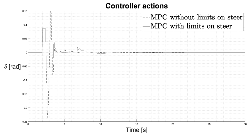
The constraints on the maximum and minimum steering angle defined by (20), slow down the controller response, as shown in Figure 5, to avoid high values of sideslip angle.

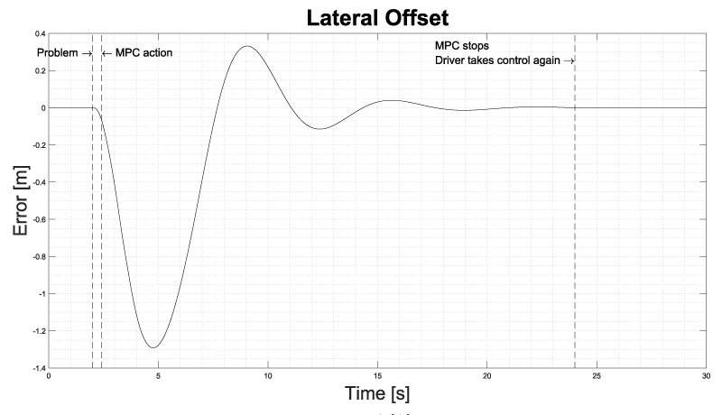
Figure 6 shows the result of the simulation in terms of lateral error in respect to the centre of the lane, which is estimated runtime in respect to the lateral offsets of the lane boundaries identified by the vision detection camera installed on the front of the vehicle.

The MPC has a prediction horizon of 15 time instants corresponding to 0.75 seconds and a control horizon of 0.01 sec.

Conclusion

A Linear Time Varying (LTV) Model Predictive Control (MPC) is presented in this paper in order to control the vehicle steering in case of anomalous events during the driving sessions. The control system estimates in real time the sideslip angle of the vehicle through a Kalman Filter and, according to specific threshold values, the controller is activated, replacing the driver, to correct the vehicle trajectory by maintaining the correct position in the lane of the road at constant speed. When a safe standard driving condition is restored, the controller gives the control back to the driver. The results show a good response of the controller which can however be improved by adding other constraints and risk assessment criteria such as overpassing lanes and prediction of the direction of the vehicle to anticipate the risk.

The model considered in this work does not take into account other important dynamics of the vehicle such as the road slope and suspensions. To include these dynamics, other considerations have to be made; in particular, it would be necessary to consider a model far more complicated and precise which requires a more powerful and efficient processor to implement a predictive control.

This research is supported by the INTERREG-ALCOTRA programme (https://www.interreg-alcotra.eu/, Programma europeo di cooperazione transfrontaliera tra Francia e Italia / Programme de coopération transfrontalière européenne entre la France et l’Italie), specifically within the SYSE2021 project num. 5665, (Centro transfrontaliero di eccellenza per la formazione in ingegneria dei sistemi / Centre d’excellence transfrontalier pour la formation en ingénierie de systèmes).

1. World Health Organization (WHO) (2018) Global Status Report on Road Safety 2018. Link: https://bit.ly/3iYQ4qp  
2. Singh S (2015) Critical reasons for crashes investigated in the national motor vehicle crash causation survey. Technical report. Link: https://bit.ly/3gc0D7M
3. Zero E, Bersani C, Zero L, Sacile R (2019) Towards real-time monitoring of fear in driving sessions. IFAC-PapersOnLine 52: 299-304. Link: https://bit.ly/3iWguZP  
4. De Nadai S, D'Incà M, Parodi F, Benza M, Trotta A, et al. (2016) Enhancing safety of transport by road by on-line monitoring of driver emotions. 2016 11th System of Systems Engineering Conference (SoSE), Kongsberg, Norway 1-4. Link: https://bit.ly/37VbRJ0
5. Zhou J (2017) Reduced complexity safety testing for adas & adf. IFAC-Papers OnLine 50: 5985-5990.
6. Graffione S, Bersani C, Sacile R, Zero E (2020) Model Predictive Control for Cooperative Insertion or Exit of a Vehicle in a Platoon. In ICINCO. 352-359. Link: https://bit.ly/3guSrPX
7. Vanderhaegen F (2012) Cooperation and learning to increase the autonomy of ADAS. Cognition, Technology  Work 14: 61-69. Link: https://bit.ly/3CXdGDO
8. Li L, Wen D, Zheng NN, Shen LC (2011) Cognitive cars: A new frontier for ADAS research. IEEE Transactions on Intelligent Transportation Systems 13: 395-407. Link: https://bit.ly/3CU2WpA  
9. Piyabongkarn D, Rajamani R, Grogg JA, Lew JY (2008) Development and experimental evaluation of a slip angle estimator for vehicle stability control. IEEE Transactions on control systems technology 17: 78-88. Link: https://bit.ly/3z16Iek
10. Hsu YHJ, Laws SM, Gerdes J (2009) Estimation of tire slip angle and friction limits using steering torque. IEEE Transactions on Control Systems Technology 18: 896-907. Link: https://bit.ly/3gd4NMv  
11. Hac A, Simpson MD (2000) Estimation of vehicle side slip angle and yaw rate. SAE transactions 1032-1038. Link: https://bit.ly/3xWx5RA  
12. Chen BC, Luan BC; Lee K (2014) Design of lane keeping system using adaptive model predictive control. In: 2014 IEEE International Conference on Automation Science and Engineering (CASE). IEEE 922-926. Link: https://bit.ly/3xZ1bUe
13. Milliken W, Milliken D (1995) Race Car Vehicle Dynamics, SAE International, Warrendale, PA. Link: https://bit.ly/2W6gr4p  
14. Rajamani R (2011) Vehicle Dynamics and Control.

© 2021 Graffione S, et al. This is an open-access article distributed under the terms of the Creative Commons Attribution License, which permits unrestricted use, distribution, and reproduction in any medium, provided the original author and source are credited.