Optimization of concentric tube continuum robot based on accuracy and overall length of the robot via genetic algorithm

Concentric Tube Continuum Robot (CTR) is a group of continuum robots which is composed of concentric tubes that can be axially translated and rotated at the base relative to one another. Their inverse kinematic is challenging due to their redundancy. On the other hand, knowledge about the inverse kinematics of the concentric-tube continuum robot is essential for control purposes. There are many solutions for reaching to a specific target point because of the redundancy of these kinds of robots. In this paper, a new method for solving the inverse kinematics of these kinds of robots is presented. The most common type of these robots consisting of three tubes is considered for this study, and the genetic algorithm technique is employed to optimize the solution of this problem. Minimum energy principle equations are used in this method. It is assumed that the robot moves in a free space, so the environment force on this robot is neglected. Also, it is supposed that the curvature of each tube remains constant along the tube. According to the results, a small error of the order 0.01mm was observed using the presented method, which is acceptable for most applications. Finally, the parameters of robot is optimized with concentration on accuracy and the overall length of the robot, which is an important parameter for stability.

Introduction

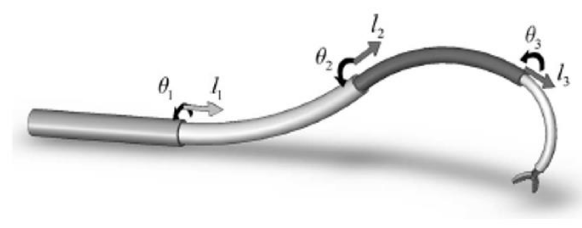
Robots can be classified into two groups: rigid-link robots and continuum robots. The advancement of science has increased robot’s applications in our daily life. In some applications continuum robots are more useful. Also, they are newer than rigid robots and they are still attractive fields of study. Concentric tube continuum robots are made up of some pre-curved tubes. Each tube can rotate and inner tubes can move through outer tubes. Figure 1 shows a concentric tube continuum robot.

In many papers, each tube is supposed to be a section of a circle with constant curvature [2-4]. In 2008, Webster, et al. presented a method for direct kinematics of concentric tube continuum robots. They assumed that active cannula is composed of sections with constant curvature [5]. In the same year, Walker, et al. represented a geometrical method for solving the inverse kinematic of concentric tube continuum robot [6]. In 2009, Webster, et al. employed Minimum Energy method to obtain the configuration of concentric tube continuum robot. [7] Webster and Rucker discussed the design and kinematics of continuum robots with constant curvature in 2010 [8]. Dupont, et al. in 2011 represented an algorithm for designing concentric tube continuum robots [9]. In 2013, Walker investigated the categorization of continuum robots [10]. In 2016, Su Li, et al. discussed the design, modeling and experimental evaluation of MRI-guided concentric tube continuum robotic system [11].

This paper concerns with the concentric tube continuum robot. The robot is made from three tubes; each tube has three parameters that should be determined. We have 9 parameters for robot and we want to reach one target that has three coordinates in space. So redundancy in this robot is sensed. Redundancy in a system cause different solutions for one answer. Therefore the inverse kinematic of this robot is challenging. Here, Genetic Algorithm optimization approach is used to solve the inverse kinematics. At first, the kinematics of concentric tube continuum robots is discussed. Then the robot is optimized for different target points. We also obtain different optimal solutions for one problem. Finally, the optimal robot with the smallest length is achieved.

Nomenclatures

e Objective function

k Curvature

l Overall length of robot

Greek symbols

μ Weighting coefficient

${\theta }^O$ Angle at initial point of a curve

${\theta }^S$ Angle at the end point of a curve

Kinematics of concentric tube continuum robots

The kinematics of the robot is based on Cosserat rod theory, in which a homogenous transfer function (g(s)) is used to describe the configuration of the robot.

$g(s)=\left(\begin{array}{cc}R(s)& P(s)\\ 0& 1\end{array}\right)\text{ (1)}$

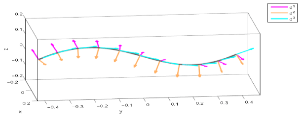
In equation (1), P(s) shows the central line of curve and R(s) shows the direction. They are functions of s, where s is the length from the base to the intended point of the robot. g(s) is shown in Figure 2.

The schematic of a curve in plane is depicted in Figure 3. The parameters in this figure are used to obtain the transfer matrix of the curve.

In order to obtain the transfer matrix for each curve, three transfer matrix should be multiplied. These matrixes are:

$T_{\text{1}}=\left[\begin{array}{cccc}\cos ({\theta }^O)& -\sin ({\theta }^O)& 0& 0\\ \sin ({\theta }^O)& \cos ({\theta }^O)& 0& 0\\ 0& 0& 1& 0\\ 0& 0& 0& 1\end{array}\right]\text{ (2)}$

T₁ shows the transfer function between the frame on curve at the initial point and the straight line

$T_{\text{2}}=\left[\begin{array}{cccc}1& 0& 0& 0\\ 0& 1& 0& d\\ 0& 0& 1& 0\\ 0& 0& 0& 1\end{array}\right]\text{ (3)}$

T₂ shows the transfer function between the initial point and last point in the straight line.

$T_{\text{3}}=\left[\begin{array}{cccc}\cos ({\theta }^S)& -\sin ({\theta }^S)& 0& 0\\ \sin ({\theta }^S)& \cos ({\theta }^S)& 0& 0\\ 0& 0& 1& 0\\ 0& 0& 0& 1\end{array}\right]\text{ (4)}$

T₃ is the transfer function between the last point on the straight line and the last point on the curve.

Finally the general transfer matrix is

$T=\left[\begin{array}{cccc}\cos ({\theta }^O+{\theta }^S)& -\sin ({\theta }^O+{\theta }^S)& 0& -d\sin ({\theta }^O)\\ \sin ({\theta }^O+{\theta }^S)& \cos ({\theta }^O+{\theta }^S)& 0& d\cos ({\theta }^O)\\ 0& 0& 1& 0\\ 0& 0& 0& 1\end{array}\right]\text{ (5)}$

The general transfer matrix T can also be written in the form below

$T=\left[\begin{array}{cccc}\cos (sk)& -\sin (sk)& 0& \frac{1}{k}[\cos (sk)-1]\\ \sin (sk)& \cos (sk)& 0& \frac{1}{k}\sin (k)\\ 0& 0& 1& 0\\ 0& 0& 0& 1\end{array}\right]\text{ (6)}$

In this paper, it is assumed that the outer tubes have larger stiffness than inner tubes. Therefore, the shape of robot in each section is the same as the outer tube in that section. This concept is depicted in Figure 4.

Optimization of the robot parameters for a specific target point with the smallest error

A concentric tube continuum robot with three tubes is considered. The optimization of robot’s parameters is adjusted to the target point a = (1, 0.5, 0.8).

The main idea for this optimization is to minimize the error. The objective function in this problem is defined as follows:

$e=\frac{1}{m_a}[{(x-x(a))}^2+{(y-y(a))}^2+{(z-z(a))}^2]\text{ (7)}$

(x, y, z) shows the coordinate of the tip and $m_a$ is obtained by the following equation:

$m_a=\sqrt{x{(a)}^2+y{(a)}^2+z{(a)}^2}\text{ (8)}$

The optimal parameters of the robot including length, curvature and rotation angle of each tube can be observed in Table 1.

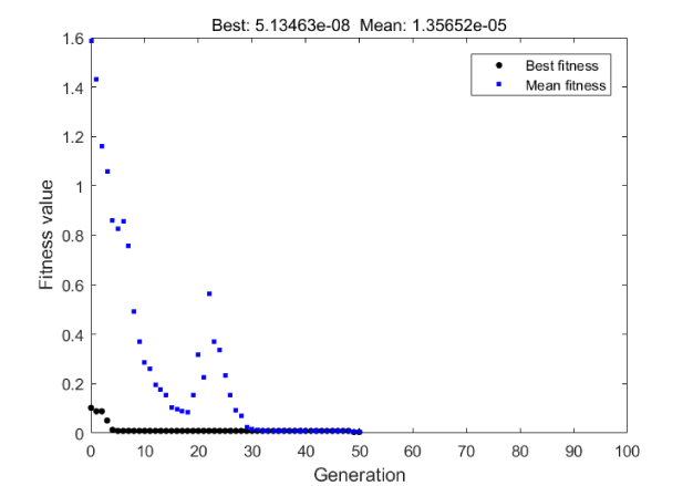
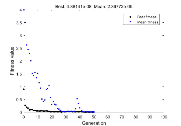
Figure 5 shows the process of the optimization in genetic algorithm for different generations. According to the results of the objective function in genetic algorithm, which is related to the best fitness in Figure 5, the error is

$error=\sqrt{e}=\sqrt{5.135}\times 0.0001=2.266\times {10}^{-4}dm=2.266\times {10}^{-2}mm$

Thus, the order of error is 0.01 mm which is very small in comparison to other methods that have the error of order 1 mm. For instance, the Error in Ref. [11] was 1.94 mm and 2.17mm.

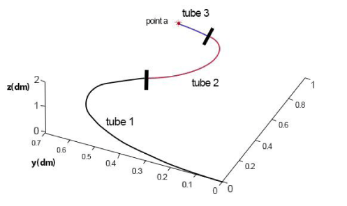
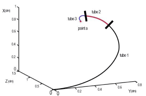
The simulation of the robot by MATLAB program is depicted in figure 6. The tubes are separated with a small line and they have different colors. Target point is shown by a red star. The first tube with the highest stiffness is black, the second tube is red and the third tube is blue.

According to redundancy of these robots, we may have different solutions for one problem. Here is another solution for the previous problem. The optimal results for the second solution are shown in Table 2.

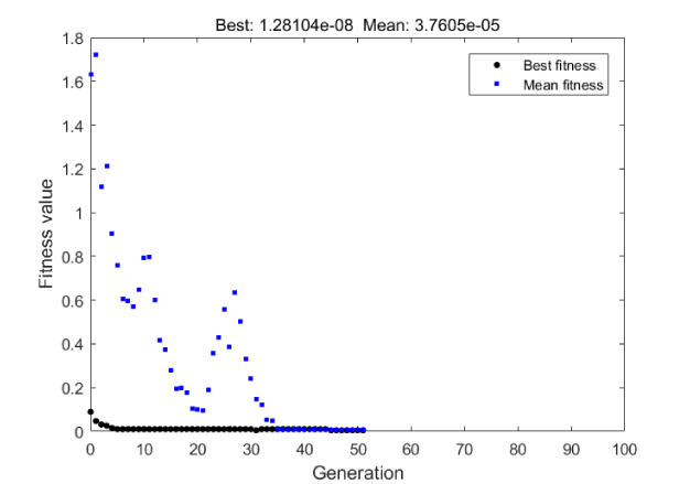
The genetic algorithm diagram which shows the process of solving according to generation is shown in Figure 7. In order to calculate the error in this problem, the best fitness for the objective function in Figure 7 is used.

$error=\sqrt{e}=\sqrt{1.281}\times 0.0001=1.132\times {10}^{-4}dm=1.132\times {10}^{-2}mm$

The simulation of the robot for the second solution can be observed in Figure 8.

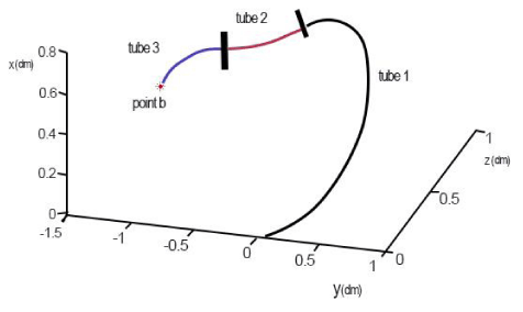
Now we want to show that this method can be a general solution and it does not depend on the target point. Thus, another target point (b) is chosen as (0.6, -1.2, 0.3). The optimal results for the target point b is written in Table 3.

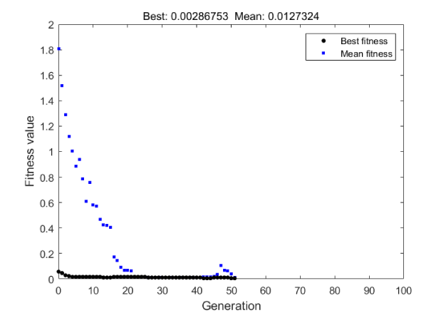
The genetic algorithm diagram for the best fitness is depicted in Figure 9. Again the error is calculated by using the best fitness for the objective function.

$error=\sqrt{e}=\sqrt{4.881}\times 0.0001=2.209\times {10}^{-4}dm=2.209\times {10}^{-2}mm$

The simulation of the optimal robot for target point b is shown in Figure 10. In this figure the tubes are also separated by small lines and different colors.

We have optimized 9 parameters in a robot simultaneously for each target point. It is assumed that the robot is consisted of three tubes. Three parameters such as length, curvature and rotation angle for each tube are optimized. The accuracy of the robot is considerably great in each case.

One of the important parameters that makes the robot more stable, is the overall length of the robot, so we have also optimized the robot for reaching a target point by the smallest length. Accordingly, a parameter is added to the objective function and it is changed into the following equation:

$\begin{array}{l}OF=\frac{1}{m_a}\left[{(x-x(a))}^2+{(y-y(a))}^2+{(z-z(a))}^2\right]\text{ (9)}\\ +\mu l\end{array}$

where, l shows the overall length of robot. Parameter μ is an optimal weighting coefficient obtained by trial and error method. The optimal result for μ is obtained as below:

$\mu =\frac{1}{500m_a}\text{ (10)}$

The optimal parameters by considering the length of robot for target point a is determined in “Table 4”

Figure 11 shows the process of solving problem with target point and for the smallest length of robot. It shows the result for each generation in Genetic Algorithm.

In Figure 12 we see that besides the small length of robot, it has a great accuracy for reaching to target point a.

By comparing Figure 12 with Figure 6 and Figure 8, the short length of robot and stability of CTR is obviously observed in Figure 12. So the Genetic Algorithm method of optimization can be used for different purposes in continuum robot problems.

Discussion

In this paper, we optimized the inverse kinematics of concentric tube continuum robots via genetic algorithm method. The problem of reaching a determined target point is discussed and the error is significantly small. In order to evaluate this method, the parameters of the robot are optimized for different target points. The problem for one target point is solved two times to show the fact that we have different optimal answers for redundant systems. In all cases the accuracy of the robot for reaching the target point is great and the order of error is 0.01mm. Finally, another quality is added to our optimization. The parameter related to overall length of robot for reaching a target point is also added to the optimization equation. When the overall length of a robot is decreased, the robot is more stable. So in the last optimization, we solved the problem for the smaller length of the robot with acceptable accuracy. In this case, the accuracy of the robot is decreased a little in comparison to the cases that the overall length of robot is not considered. But its error is still negligible. The stability is a very important parameter in a robot, so the last optimization has its special benefit. Using each optimization form relates to the situation and the application of robot and choosing the best equation relates to the case.

Conclusions

In this paper, the main goal is to reach to a target point with a high accuracy. 9 parameters are optimized simultaneously for each target point and this is one of the advantages of this method. According to the obtained results, the accuracy is great and the error is in the order of 0.01mm; which is very small in comparison to others. Thus, the genetic algorithm can be a good optimization solver for continuum robots because of its multi objective premium.

1. Dupont PE, Lock J, Itkowitz B, Butlar E (2010) Design and Control of Concentric-Tube Robots. IEEE Transactions on Robotics 26. Link: https://bit.ly/2XadNsk
2. Xu K, Simaan N (2008) An investigation of the intrinsic force sensing capabilities of continuum robots. IEEE Transactions on Robotics 24: 576-587. Link: https://bit.ly/2BGPr1F
3. Webster RJ, Romano JM, Cowan NJ (2009) Mechanics of Precurved-Tube Continuum Robots. IEEE Transactions on Robotics 25: 67-78. Link: https://bit.ly/3fd9IK3
4. Neppalli S, Jones BA (2007) Design, construction and analysis of a continuum Robot. IEEE/RSJ International Conference on Intelligent Robots and Systems 1503-1507. Link: https://bit.ly/3jUjqod
5. Webster RJ, Romano JM, Cowan NJ (2008) Kinematics and Calibration of Active Cannulas. IEEE International Conference on Robotics and Automation, Pasadena, CA, USA. Link: https://bit.ly/3faVA44
6. Neppalli S, Csecsits MA, Jones BA, Walker I (2008) A Geometrical Approach to Inverse Kinematics for Continuum Manipulatores. IEEE/RSJ International Conference on Intelligent Robots and Systems. Link: https://bit.ly/2P91jg6
7. Jones AB, Gray RL, Turlapati K (2009) Three Dimentional Statics for continuum robotics. IEEE/RSJ International Conference on Intelligent Robots and Systems 2659-2664. Link: https://bit.ly/2P91Gau
8. Webster RJ, Jones BA (2010) Design and Kinematic Modeling of Constant Curvature Continuum Robots: A Review. International Journal of Robotics Research 29. Link: https://bit.ly/2D54rHj
9. Anor T, Madsen JR, Pierre D (2011) Algorithms for Design of Continuum Robots Using the Concentric Tubes Approach: A Neurosurgical Example. IEEE International Conference on Robotics and Automation, Shanghai International Conference Center Shanghai, China. Link: https://bit.ly/3hULG8t
10. Walker ID (2013) Continuous Backbone “continuum” Robot Manipulator. International Scholarly Research Notices 2013: 726506. Link: https://bit.ly/2D3zW4v
11. Su H, Li G, Caleb Rucker D, Webster RJ, Fischer GJ (2016) A Concentric Tube Continuum Robot with Piezoelectric Actuation for MRI-Guided Closed-Loop Targeting. Annals of Biomedical Engineering 44: 2863-2873. Link: https://bit.ly/3gk0Y6o
12. Pascal J, Sigrid L, Joachim L, Michael O (2010) A discrete mechanics approach to Cosserat rod theory, Part: static equilibria. CA, USA, International Journal for Numerical Methods in Engineering 85: 31-60. Link: https://bit.ly/3fhpzaq

© 2020 Davarpanah A, et al. This is an open-access article distributed under the terms of the Creative Commons Attribution License, which permits unrestricted use, distribution, and reproduction in any medium, provided the original author and source are credited.