Complex network reveals the spatiotemporal pattern of summer extreme precipitation in Eastern China

In this study, complex networks were constructed based on the synchronization of summer extreme precipitation events (SEPEs) in eastern China. Then, a detailed analysis of spatiotemporal patterns of SEPEs and the relationship between SEPEs in eastern China with the eastern Asian monsoon was presented. The results showed that (1) the event synchronization is low in the coastal region but high in the inland region; (2) the intensity of the monsoon varies at different phases of summer and the area and intensity of the monsoon's influence on the summer extreme rainfall events were different. In conclusion, this study provides valuable insights to reveal the influence of monsoon strength on SEPEs in different regions of China.

Introduction

With the intensification of global warming, the frequency of extreme rainfall events in summer has increased, posing a major threat to the production and life of human society. Therefore, there are more and more studies on extreme rainfall events. Complex networks have facilitated the research on extreme rainfall events.

Complex networks are composed of node sets and edge sets representing the situation of links between nodes, using weights to represent the different strengths of the existence of links and characterizing time series networks as directed and weighted networks to concretize abstract data. The empirical studies, models and approaches analyzed to obtain that real networks are far from random, deepening the understanding of real networks and advancing the theory of complex networks [1]. The methodology of complex networks has become a significant mathematical tool in the study of various disciplines in the natural sciences as well as the social sciences in recent years. Complex networks have played an extremely essential role in the study of climate networks, Tsonis used complex network theory to identify the community structure in the climate system [2], Steinhaeuse used complex network theory to identify the linkages between different regional climate phenomena and Swanson and Tsonis used complex network theory to identify the linkages between different regional climate phenomena. Swanson and Tsonis used complex network theory to discover new dynamical mechanisms of major climate changes [3]. In this paper, a complex network method is used to study the influence of monsoon strength on rainfall patterns over Eastern China.

Climate networks are networks that apply the idea of complex networks to climate science, with geographic location as nodes of the network and the degree of similarity between time series represents the network of links and their strength. Climate networks can be used to study the interrelationships between various locations around the globe to further understand the causes behind many of the meteorological events in the global climate system. In this study, the geographical locations of the central and northern regions of China are used as the nodes of the network, and the synoptic strength between the summer extreme rainfall time series is used to construct connections to form a climate network, as a way to study the influence of SEPEs on a day-scale by the strength of the monsoon.

With the intensification of global warming, more and more studies on extreme rainfall in China have been conducted in recent years and many research results have been obtained. From these studies, it is clear that the temporal trend of total national rainfall in recent years is not significant, but the number of days of heavy rainfall nationwide has increased considerably and the intensity of rainfall has increased remarkably.

In this study, complex networks were constructed based on the synchronization of summer extreme precipitation events (SEPEs) in eastern China. The effects of monsoon strength on SEPEs in the first half of summer and the second half of summer were compared by analyzing the network attributes. Therefore, this paper collects statistics on extreme rainfall events in China in summer, analyzes the impact of monsoon strength on extreme rainfall events on the time scale, to prepare for the causes and predictions of subsequent extreme rainfall events and then reduce the impact of extreme rainfall events on people's production and life.

Data and methodology

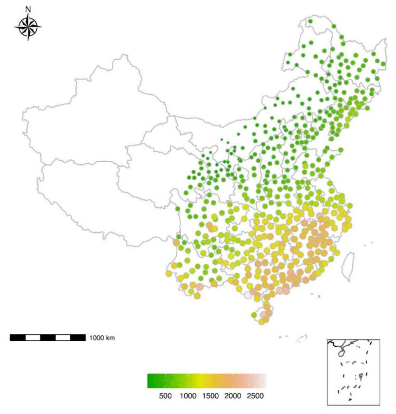
The daily precipitation dataset (1951–2013) that was provided by the National Meteorological Information Center (NMIC) of the China Meteorological Administration (CMA) was used to extract extreme precipitation time series. The dataset was open to registered users and could be accessed from the following official website https://data.cma.cn/. We are only interested in the extreme precipitation events in eastern China since the western part of China is dry. In this study, daily precipitation time series from 243 sites were adopted for the construction of the climate networks (Figure 1).

Figure 1: The distribution of annual average rainfall at selected grid points.

Event synchronization is applied for complex network construction and the specific process is divided into the following three steps. Firstly, the rainfall events for each precipitation time series are defined based on the 75th percentile threshold of daily rainfall in the five months from May to September in China and then the synchronization matrix Q_ij and the delay matrix q_ij are calculated. Secondly, based on the matrix characteristics, undirected or directed links are established, thus transforming the event-synchronized climate network into a matrix. Finally, the network measurements are estimated from the adjacency matrix.

Event synchronization is described in [4], which can be used to compute nonlinear relationships between time series at selected sites. The event synchronization method is simplified in [5], which allows the method to be more widely used. The event synchronization method used in this paper is briefly introduced: two sites i and j are arbitrarily selected to allow the existence of a time difference between the occurrence of extreme rainfall events. In a certain period, the degree of extreme rainfall events is measured by calculating the number of overlapping extreme rainfall events.

This variable time lag is defined as follows:

${\tau }_{lm}^{ij}=min\left\{\frac{t_{l+1}^i-t_l^i,t_l^i-t_{l-1}^i,t_{m+1}^j-t_m^j,t_m^j-t_{m-1}^j,}{2}\right\}\text{ (1)}$

Where $t_l^i$ denotes the time at which event i occurs at site i(i = 1,2,…,s_i), $t_m^j$ denotes the time at which event m occurs at site j(j = 1,2,…,s_i) and ${\tau }_{lm}^{ij}$ denotes the dynamic time delay between event i and event m. s_i. And s_j denote the total number of such events located at site i and j, respectively.

The following defines c(i|j)as the number of events that occur first at site j and then at site i:

$c\left(i|j\right)={\displaystyle \sum }_{l=1}^{s_i}{\displaystyle \sum }_{m=1}^{s_j}{J}_{ij} \text{ (2)}$

where

$J_{ij}=\left\{\begin{array}{c}1 if 0<t_l^i-t_m^j<{\tau }_{lm}^{ij}\\ 0.5 if t_l^i=t_m^j \\ 0 if otherwise\end{array}\right\}\text{ (3)}$

Based on the definition of c(i|j), c(j|i) can be similarly obtained. Therefore, we define

$Q_{ij}=\frac{c\left(i\text{|}j\right)+c(j|i)}{\sqrt{s_i{s}_j}}\text{ (4)}$

$q_{ij}=\frac{c\left(i\text{|}j\right)-c(j|i)}{\sqrt{s_i{s}_j}}\text{ (5)}$

Q_ij measures the strength of synchronization of SEPEs between two sites at sites i and j and q_ij measures the delay behavior and. $-1\le q\le 1$

Based on the synchronization matrix Q_ij and the delay matrix q_ij, undirected and directed connections can be established to construct undirected and directed complex networks, respectively. In the process of establishing the links, we set the threshold criteria to select meaningful links. In an undirected complex network, the synchronization matrix can be transformed into an adjacency matrix as follows:

$A_{ij}^Q=\left\{\begin{array}{c}1 if Q_{ij}>\theta \\ 0 if otherwise\end{array}\right\}\text{ (6)}$

In a directed complex network, the delay matrix can be transformed into an adjacency matrix as follows:

$A_{ij}^q=\left\{\begin{array}{c}1 if \left|q_{ij}\right|>\delta \\ 0 if otherwise\end{array}\right\}\text{ (7)}$

Where θ and δ denote the threshold criteria we set, respectively.

In summary, the adjacency matrix in an undirected complex network (directed complex network) can be constructed by the synchronization matrix Q_ij (the delay matrix q_ij). The adjacency matrix $A_{ij}^Q$ contains the synchronization intensity information between extreme rainfall events, while the adjacency matrix $A_{ij}^q$ contains the direction information along with the synchronization intensity. In undirected networks, the relevant network coefficients, such as degree, average link distance and clustering can be further calculated from the adjacency matrix. In a directed complex network, relevant network coefficients can be further computed from the adjacency matrix, such as local network flow and network links.

In this study, extreme rainfall events in the Chinese region are considered, thus, for a network with boundaries, the boundary effect has an important impact on them. Therefore, by generating a fixed number of spatially embedded random networks (SERN) as surrogates with the same positions as the original network and the same link probability with the same spatial connection length, the measurements in this SERN are used as boundary effect estimates, and the metrics are averaged over the set of surrogates to improve the estimation of boundary effect in a particular network metric. The estimate of the corrected network is calculated by subtracting the estimate of the network measurement from the original network measurement so that the spatial bias due to artificial boundaries is significantly eliminated after correction [6]. The construction of the complex network was programmed using the statistical computing environment R, and the statistical analysis of the network was implemented using the R-package “igraph”. The scripts used in the study could be accessed from the corresponding author via email.

Results

Based on complex network theory, the definition of the relevant network coefficients and their practical significance are specified.

Degree and degree distribution

The degree is the number of edges connecting a point with other points. The degree at i is denoted by k_i and the degree of the undirected network is formulated as:

$k_i={\displaystyle \sum }_{j=1}^N{A}_{ij}\text{ (8)}$

Where N is the number of vertices and A_ij is the adjacency matrix for the undirected network.

The degree in the directed network is divided into the outgoing connections and the incoming connections, where the in-degree is performed as follows:

$k_i^{in}={\displaystyle \sum }_{j=1}^N{A}_{ij}\text{ (9)}$

The outdegree is defined as:

$k_j^{out}={\displaystyle \sum }_{i=1}^N{A}_{ij}\text{ (10)}$

Where N is the number of vertices and A_ij is the adjacency matrix for the directed network.

MJJ indicates May 1-July 15 and JAS represents July 16-September 30 (Figure 2). This figure depicts the spatial regions associated with the degree distribution [7]. The summer season is divided into two time periods for comparative analysis, to better understand the effect of monsoon variability on rainfall. The spatial distribution of degrees visualizes the synchronization of summer extreme rainfall. It can be seen from Figure 2 that the degree of the inland region (red region) is relatively high, indicating that the event synchronization is high in this region, that is, the spatial synchronization of extreme summer rainfall is high; in the coastal region, the degree is generally smaller, which indicates that the spatial synchronization of summer extreme rainfall is low. The degree of the northern region is relatively large, but the degree of the southern region is relatively small, and the degree distribution from MJJ to JAS shifts roughly upward as a whole, indicating that the influence area of the summer monsoon is increasing.

Figure 2: The distribution of the correction degree after removing the boundary effect.

Average link distance

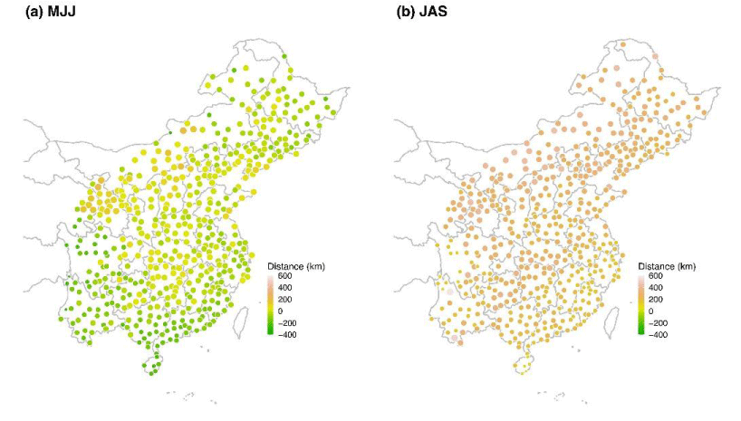
In this study, the average link distance at each site is calculated and the modified average link distance distribution as shown in Figure 3 is obtained based on the consideration of boundary effects. If there is a connection between sites, the formula for spherical earth projected on to plane can be used to calculate the distance between grid points i and j and the formula is:

Figure 3: The modified average link distance distribution.

$L_{ij}=R\sqrt{{\left(\delta {\varnothing }_{ij}\right)}^2+{\left(\cos \left({\varnothing }_m\right)\delta {\lambda }_{ij}\right)}^2}\text{ (11)}$

Where δφ_ij denotes the difference in latitude between sites i and j, δλ_ij denotes the difference in longitude between sites i and j, φ_m denotes the mean value of latitude between sites i and j and R denotes the radius of the earth.

This metric can concretize the abstracted spatial metric and facilitate our understanding of the impact of monsoons on extreme rainfall events. From Figure 3, we can see that the average link distances in the southwest, south and northeast regions are small during the MJJ period, which means that these regions are not only influenced by the monsoon but also affected by the topography and other factors. The main reason for the small link distance is that the monsoon is blocked by high mountains just after it enters the land, which indicates the relatively low strength of the monsoon. Overall, the average link distance in most parts of central and eastern China is less than 200Km during the MJJ period, but greater than 200Km during the JAS period, and the average link distance increased as a whole, thus revealing that the influence range of monsoon activity became larger, and the intensity of monsoon activity increases, that is, the extreme rainfall events in summer are increasingly influenced by monsoon activity as a proportion. The comparison of the mean link distance during the MJJ and JAS periods reveals that the influencing factors of extreme rainfall events in summer tend to be dominated by monsoon activity as the monsoon activity intensifies.

Clustering of SEPEs

Relevant features of the system can be revealed by the topology of the network [8,9] and communities are one of these features [10]. Communities represent tightly connected groups of nodes with only a few connections between node groups. Interaction networks are networks with a distinct community structure, with communities or clusters identified by community detection algorithms as subnetworks [11]. In this study, we follow the scale of days and use the Edge-Betweenness algorithm for multi-scale community detection to identify the different communities where SEPEs occur.

In order to clearly distinguish the community structure, it is necessary to remove the critical connections between two different communities and therefore the concept of Edge-Betweenness is proposed to quantify the "criticality" of the links. The edge betweenness represents the percentage of all shortest paths through the edge out of all shortest paths so that a larger edge betweenness indicates the existence of a critical link between two different communities, through which the two communities interact. Thus, by severing these critical connections, a distinct network structure can be distinguished (Figure 4).

Figure 4: Clustering of SEPEs on the scale of days.

In the MJJ period and the JAS period, which have different numbers of communities, the number of communities has decreased significantly. The southern and southeastern regions of China merged from multiple communities during the MJJ to one community during the JAS period, indicating that the monsoon intensity increased. In contrast, the regional communities of Yunnan do not change, mainly because of the existence of the Yunnan-Guizhou plateau, which hinders monsoon activity. During the period from MJJ to JAS, a separate region is formed in Zhejiang and southern Jiangsu because the region is the Yangtze River Delta, and the distribution of lakes, rivers and other water areas affects the extreme rainfall events in summer. This shows that the intensity of monsoon activity tends to increase in summer. However, quantifying the driving weather patterns corresponding to each of the SEPE regimes and how these regimes interact with each other is a topic of future research [12].

Local network flux

The degree in a directed complex network is divided into outdegree and indegree, where outdegree indicates the number of outgoing connections from a site and indegree represents the number of incoming connections into the specified site. In this paper, we define the local network flow as the difference between the indegree and the outdegree:

$\Delta k=k^{in}-k^{out}\text{ (12)}$

Where kⁱⁿ denotes indegree in a directed complex network and k^out denotes outdegree in a directed complex network. According to the definition of local network flow, it can be used to characterize the direction of water vapor transport in the network and the evolution of extreme rainfall events in summer. A high positive value indicates that the incoming connection is greater than the outgoing connection, and the moisture accumulates at the regions, which are moisture sinks; a high negative value indicates that the outdegree is greater than the indegree and the regions are closer to the moisture sources. Extreme rainfall events are usually generated by convective rainfall [13] and thus mesoscale convective systems (MCS) play an important role in generating these rainfall amounts [14,15]. Thus, the identified sinks and sources can be correlated with the spatial pattern of MCS within the Chinese region.

As observed in Figure 5, red areas are generally arid areas, which are moisture sinks; purple areas are generally coastal areas, which are moisture sources. During the period from MJJ to JAS, ∆k increased significantly in the southeast region and the eastern coastal region, which is due to the increase of water vapor brought by the enhanced southeast monsoon; while ∆k does not change obviously in the southwest, one is due to the southwest monsoon which almost does not change much, and the other is due to the effect of topography; for the north-central region of China is deep inland and less influenced by the monsoon and belongs to the non-monsoon area, so there is no significant change in ∆k. From the above analysis, ∆k reveals from another perspective that the monsoon activity is stronger in the second half of Chinese summer than in the first half.

Figure 5: Local network flux obtained from directed networks.

Visualising links of complex networks for the selected region

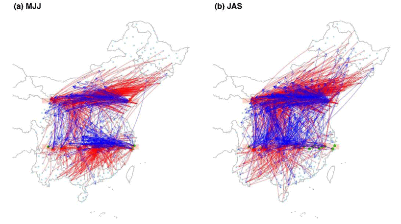
It can be seen from the figure that the density of links is significantly enhanced from the MJJ to JAS period, with more typhoons in the southeast coastal areas and more waters in the Yangtze and Yellow River basins such as lakes and tributaries, which results in dense water vapor exchange. Due to the enhanced monsoon, every region is affected and therefore rainfall events occur and the synchronization of extreme rainfall events increases, resulting in an enhanced density of links. The connection areas between the Yangtze River basin and the Yellow River basin become extensive during MJJ-JAS as shown in Figure 6, which indicates that the area affected by the enhanced monsoon activity becomes increasingly.

Figure 6: The links of the selected Yangtze River basin (latitude: 28.5°-29.5°) and Yellow River basin (latitude: 37.5°-38.5°), with red links indicating inputs and blue links indicating outputs.

Conclusions

The complex network of summer extreme rainfall in China was constructed by the event synchronization method, and the influence of monsoon strength on SEPEs was analyzed by using the structural characteristics of the complex network. The main conclusions are as follows:

(1) The event synchronization method establishes the link between sites from the perspective of time synchronization of events and the constructed complex network of extreme rainfall is a two-way network, which contains both link strength information (reflecting the synchronization of summer extreme precipitation events among grid points) and direction information (reflecting the temporal sequence of summer extreme rainfall events among sites).

(2) The spatial distribution of the characteristic quantity-degree of the complex network structure indicates that the spatial synchronization of extreme summer rainfall is gradually increasing from the coastal regions to the inland regions. The low average link distance in the southeast, as well as southwest regions of China and the high average link distance in the northern land regions, reveal that the association space is large in the inland regions and small in the coastal regions. A multi-scale community detection based on the Edge-Betweenness algorithm is used to identify different communities where summer extreme rainfall events occur, and the influencing factors of each community are specifically analyzed. Meanwhile, the spatial distribution of network flow reveals that the monsoon activity is stronger in the second half of summer in China than in the first half, which also provides a new method to study the direction of water vapor transmission transport.

In this work, the changes in extreme rainfall events in Chinese regions during the pre-summer and post-summer time periods reveal the changes in monsoon strength from the perspective of complex networks. However, the extreme rainfall processes in Chinese summers are very complex and influenced by various factors such as water vapor transport, monsoon, topography, weather systems, etc. Therefore, a comprehensive understanding of the specific causes of extreme rainfall in China and accurate prediction of regional rainfall events in China are important topics for the future.

1. Albert R, Barabási AL. Statistical mechanics of complex networks. Rev Mod Phys. 2002; 74: 47-97.
2. Tsonis AA, Wang G, Swanson KL. Community structure and dynamics in climate networks. Clim Dyn. 2011; 37: 933–940.
3. Swanson KL, Tsonis AA. Has the climate recently shifted? Geophys Res Lett. 2009; 36: L06711.
4. Qiao P, Gong Z, Liu W, Zhang Y, Feng G, Dong W. Extreme rainfall synchronization network between Southwest China and Asia–Pacific region. Clim Dyn. 2021; 57: 3207-3221.
5. Quian Quiroga R, Kreuz T, Grassberger P. Event synchronization: a simple and fast method to measure synchronicity and time delay patterns. Phys Rev E Stat Nonlin Soft Matter Phys. 2002 Oct;66(4 Pt 1):041904. doi: 10.1103/PhysRevE.66.041904. Epub 2002 Oct 15. PMID: 12443232.
6. Rheinwalt A, Marwanl N, Kurths J, Werner P, Gerstengarbel FW. Boundary effects in network measures of spatially embedded networks. EPL. 2012; 100(2):28002.
7. Malik N, Bookhagen B, Marwan N, Kurths J. Analysis of spatial and temporal extreme monsoonal rainfall over South Asia using complex networks. Clim Dyn. 2012; 39: 971–987.
8. Albert R, Barabási AL. Statistical mechanics of complex networks. Rev Mod Phys. 2002; 74: 1–54.
9. Strogatz SH. Exploring complex networks. Nature. 2001; 410: 268–276.
10. Newman ME, Girvan M. Finding and evaluating community structure in networks. Phys Rev E Stat Nonlin Soft Matter Phys. 2004 Feb;69(2 Pt 2):026113. doi: 10.1103/PhysRevE.69.026113. Epub 2004 Feb 26. PMID: 14995526.
11. Fortunato S. Community detection in graphs. Phys Rep. 2010; 486: 75-174.
12. Mondal S, Mishra AK, Leung LR. Spatiotemporal Characteristics and Propagation of Summer Extreme Precipitation Events Over United States: A Complex Network Analysis. Geophys Res Lett. 2020; 47: 1668257.
13. Schumacher C, Houze RA. Stratiform Rain in the Tropics as Seen by the TRMM Precipitation Radar. J. Clim. 2003; 16:1739-1756.
14. Johnson RH. Mesoscale processes. In: Wang B (ed) The Asian monsoon. Springer, 2006; 8: 331-356.
15. Houze RA, Wilton DC, Smull BF. Monsoon convection in the Himalayan region as seen by the TRMM Precipitation Radar. QJR Meteorol Soc. 2007;133: 1389–1411.