Lissajous curves with a finite sum of prime number frequencies

The Ulam spiral inspired us to calculate and present Lissajous curves where the orthogonally added functions are a finite sum of sinus and cosines functions with consecutive prime number frequencies.

We may say that prime numbers fascinates mankind for more than two thousand years. The scientific literature of number theory - which in great part deals with prime - is enormous and fills libraries. Number theory is not our field of interest at all, so it is not our duty to give any kind of overview of the field, therefore we just mention two works about primes [1,2]. (Our scientific interest is laser-matter interaction [3] and self-similar solutions of non-linear partial differential equations of flow systems [4].) We just would like to show a tiny idea about primes which might be interesting to the experts. Two starting points that gave as the idea. The first is the Ulam spiral which was found by Stanislaw Ulam in 1967 [5]. The left figure in Figure 1 shows how the spiral is defined, the middle figure shows how the prime numbers are distributed among the first 400 natural numbers, and the last right figure presents the prime distribution on a much larger scale. The primes are represented with dark dots, spots, and with short lines. It is evident, that there is a non-trivial correlation of primes even on large scales in this representation.

Figure 1: The Ulam spiral. The left figure is just the definition of the spiral, the middle figure shows the prime distributions among the first 400 natural numbers, the right figure presents the large scale distribution of primes in the Ulam spiral. Figures were taken from the english Wikipedia page of the Ulam spiral.

Our second starting point is the definition of Lissajous (or Bowditch) curves [6] which are a well-known object for physicists. The parametric formula of the curve reads

$x\mathrm{<mo\; stretchy="false">(</mo>}t\mathrm{<mo\; stretchy="false">)</mo><mo>=</mo>}sin\mathrm{<mo\; stretchy="false">(</mo>}a\cdot t+\delta \mathrm{<mo\; stretchy="false">)</mo>,}$

$y\mathrm{<mo\; stretchy="false">(</mo>}t\mathrm{<mo\; stretchy="false">)</mo><mo>=</mo>}cos\mathrm{<mo\; stretchy="false">(</mo>}b\cdot t\mathrm{<mo\; stretchy="false">)</mo>,}\text{ (1)}$

where 'a', and 'b' are the relative frequencies and $\delta$ is the phase between the two oscillations. Figure 2 presents three classical Lissajous curves with various relative frequencies and phases between the two trigonometric functions. The length of the corresponding parametric curve is defined as

Figure 2: Three classical Lissajous curves. The three parameter sets (from left to right) are $\mathrm{<mo\; stretchy="false">(</mo>}a\mathrm{<mo>=</mo>1,}\delta \mathrm{<mo>=</mo>}\frac{\pi }{2}\mathrm{,}b\mathrm{<mo>=</mo>2<mo\; stretchy="false">)</mo>}$ , $\mathrm{<mo\; stretchy="false">(</mo>}a\mathrm{<mo>=</mo>3,}\delta \mathrm{<mo>=</mo>}\frac{\pi }{2}\mathrm{,}b\mathrm{<mo>=</mo>2<mo\; stretchy="false">)</mo>,}$ and $\mathrm{<mo\; stretchy="false">(</mo>}a\mathrm{<mo>=</mo>3,}\delta \mathrm{<mo>=</mo>}\frac{\pi }{4}\mathrm{,}b\mathrm{<mo>=</mo>4<mo\; stretchy="false">)</mo>}$ and

$L\mathrm{<mo>=</mo>}{\displaystyle {\int }_0^{2\pi }}\sqrt{\dot{x}{\mathrm{<mo\; stretchy="false">(</mo>}t\mathrm{<mo\; stretchy="false">)</mo>}}^2+\dot{y}{\mathrm{<mo\; stretchy="false">(</mo>}t\mathrm{<mo\; stretchy="false">)</mo>}}^2}dt\mathrm{,}\text{ (2)}$

where prime means derivation with respect to the parameter t. With this formula, it is trivial to get back the circumference of a unit circle. It is also clear that the length of various Lissajous curves is proportional to $\pi$ . Differential geometrical analysis helps to derive and study additional parameters of the curve.

Let's try to image the distribution of primes somehow with the help of the Lissajous curves.

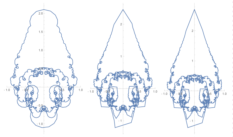
We applied the next parametric formula for the curve

$x\mathrm{<mo\; stretchy="false">(</mo>}t\mathrm{<mo\; stretchy="false">)</mo><mo>=</mo>}{\displaystyle \sum _{i\mathrm{<mo>=</mo>1}}^N}\frac{sin\mathrm{<mo\; stretchy="false">(</mo>}{a}_i\cdot t\mathrm{<mo\; stretchy="false">)</mo>}}{a_i}\mathrm{,}$

$y\mathrm{<mo\; stretchy="false">(</mo>}t\mathrm{<mo\; stretchy="false">)</mo><mo>=</mo>}{\displaystyle \sum _{i\mathrm{<mo>=</mo>1}}^N}\frac{cos\mathrm{<mo\; stretchy="false">(</mo>}{a}_i\cdot t\mathrm{<mo\; stretchy="false">)</mo>}}{a_i}\mathrm{,}\text{ (3)}$

where $a_i$ s are the first N prime numbers. Figure 3 shows the Lissajous curves for $N\mathrm{<mo>=</mo>100,1000}$ and 5000 where the last primes are 541,7919 and 104729. To achieve a finite surface for the Lissajous curve we divide the sum of sinus and cosines functions with the corresponding prime number. Note, the slight left-right symmetry breaking of the curves. These are our starting points, of course, the applied curves can be changed in numerous ways.

Figure 3: Our Lissajous curves with different kind of finite Fourier sums with prime number frequencies. From left to right, the sum of the first 100, 1000 and 5000 primes were taken.

In the second case, Figure 4 presents two curves where only the second neighbor primes are considered to the 'x' and 'y' coordinates such as 2,5,11 and 3,7,13. Note, with the much quicker convergence, it is not possible to see the differences between the two figures with naked eyes. We tried to modify Eq. (3) with additional logarithmic, square root, or power law functions of the argument of the sinus and cosines function to create a much more internal structure of the curves at a larger number of primes. Unfortunately in vain. This is the present endpoint of our idea and analysis. (The presented calculations and figures were evaluated with Maple 12.) It can happen that our toy model might give an idea for such kind of further investigations.

Figure 4: Our Lissajous curves with different kind of finite Fourier sums with prime number frequencies. From left to right, the sum of the first 100 and 1000 second neighboring primes were taken.

1. Maier H, Schleich WP (2009) Prime Numbers 101, Wiley Interscience.
2. Estermann T (1952) Introduction to Modern Prime Number Theory, Cambridge the University Press.
3. Barna IF, Pocsai MA, Varró S (2018) Eur. Phys. J. Appl. Phys. 84, 20101.
4. Barna IF, Pocsai MA, Mátyás L (2020) Fluid. Dyn. Res. 52, 015515.
5. Stein M, Ulam SM (1967) "An Observation on the Distribution of Primes." American Mathematical Monthly 74, 43.
6. Lawrence D (1972) A Cataloge of Special Plane Curves, (Page 178.) Dover Publication.