From Engle & Granger model to Johansen model for a more accurate photovoltaic power output forecast

The French government has recently decided to increase the Photovoltaic (PV) capacities to reach 35GW by 2028 in all french territories, the European territory, and overseas territories such as Reunion Island in the Indian Ocean. However, integrating growing numbers of PV power installations and microgrids onto the grid can result in larger-than-expected fluctuations in grid frequency. This is due to PV power output that is not only a function of the operating temperature and solar irradiation but also of other environmental parameters. In this paper, only two environmental parameters are considered in the European zone and when the Engle & Granger statistical method is used, a relationship between variables such as photovoltaic power output and solar irradiation at a different level is obtained. The final relationship without suspicious heteroscedasticity is determined. The model is formulated on the basis of photovoltaic real conditions statistical approach and is more realistic than steady approach models. The Engle & Granger method does not distinguish several cointegration relationships when more variables are considered. For the overseas zone, we added other measured environmental variables and applied a more robust statistical method known as the Johansen vector error correction model (VECM) cointegration approach. In the VECM model, for N explanatory variables and for N > 2, we established a long-run equilibrium relationship that has been tested and the outcome is more than reliable when comparing the model to measured data.

Introduction

Renewable energies [1,2] are strongly developed to decarbonize our way of life in the energy sector and electricity production. The goal of this research is to contribute to the improvement of the short and medium-term predictability of Photovoltaic (PV) power production. The study is based on an analysis and prediction model (b) of PV production, involving spatial and temporal meteorological parameters. Power output (P) from PV systems in outdoor conditions is substantially influenced by climatic parameters such as solar irradiance (G) and module temperature(T). Integrating growing numbers of PV power installations and microgrids [2] onto the grid can result in larger-than-expected fluctuations in grid frequency. This is due to PV power output that is not the only function of the operating temperature and solar irradiation but also of other environmental parameters. In this paper, the geographical distribution of PV output considering the module temperature effect and irradiation and other environmental parameters on PV system performance is considered in two different French territories: the European territory and an overseas territory such as Reunion Island in the Indian Ocean. The goal is to determine a linear relationship between PV power output and the environmental parameters from time series data.

For the European territory, we investigated rigorous statistical methods such as Engle & Granger (EG) [3,4], for stationary series to determine the estimate regression between variables P, G & T. In the EG method, when PV explanatory variables are nonstationary then the first difference study must be applied as the first difference transformation may make a nonstationary time series to become a stationary series to reach the final PV equation. Moreover, when outliers are suspected in the model, the EG method is put forward to determine the most appropriate model. We investigated the dependent variable P on explanatory variables such as G and T. We first applied the Augmented Dickey & Fuller (ADF) [5,6], to our time series. The ADF test is a unit root test for stationarity. In this study, a visual diagnosis tool known as correlogram [7,8], is used to identify the first step for stationary test computing the autocorrelation function and the partial autocorrelation function. When serial correlation in residuals is detected, we first applied the Goldfeld-Quandt(GQ) [9], test when heteroscedastic variance is related in variables followed by the Durbin Watson (DW) [3] test in the regression model.

The downside of the EG method is that it does not distinguish several cointegration relationships for N simultaneous variables invoking up to N-1 cointegration relations. To overthrow such a situation, a more robust statistical method is suggested known as the Johansen vector error correction model (VECM) [10-12]. The Johansen test can be considered as a multivariate generalization of the ADF test, but the former is a strategic test that makes it possible to estimate all cointegrating vectors when more than two variables are considered. For the overseas and tropical zone, the Johansen VECM model is well adapted and we considered more explanatory variables such as wind speed(Wind) and humidity (Humi) that are added to G & T.

Therefore, this paper is divided into two parts comparing the model obtained to measured data for the two French territories: the European zone and the Tropical zone.

For the European zone, the EG model is determined for data from the GREEN platform of the Physics department of the University of Lorraine in Metz in northeast France. The PV design of the GREEN platform [13] is a grid-connected system. Six PV polycrystalline modules of SCHÜCO technologies are connected in a series wiring pattern and mounted on the south-southeast vertical wall of the platform building. Each module has a peak power of 205 Wp, a tilt angle of 60°, low ventilation, and is connected to an SCHÜCO inverter for a power level up to 1 kW. For the European zone, only data such as PV power out, solar radiation, and module temperature should be considered in the EG method to determine the estimated regression between these variables. The resulting model is then compared to real data to show a good agreement between the model and measured PV output data.

For the tropical zone on Reunion island in the Indian Ocean, the Johansen VECM model is performed to determine the regression relationship. The PV system in Reunion island is a grid-connected system. The modules that make up the PV plant are at a tilted angle of 21°, the same as Reunion Island latitude. The polycrystalline PV module of 180W each is equipped with solar irradiance, cell temperature, and wind and humidity sensors.

Other environmental parameters such as wind speed and humidity are considered in addition to solar radiation and module temperature for the tropical zone. The EG method is not suitable for the tropical zone as more than 2 explanatory variables are considered, therefore the VECM model should be considered. The final long-term relationship obtained is compared to the recorded power output in real outdoor conditions.

This paper is organized as follows. Section 2 is the outline of correlograms for solar irradiance as well as its first difference to identify the stationary series. Still in that section, as the European zone is mainly focused on the Engle & Granger method, the EG principle is explained and applied to PV data from the Green platform in Metz. Section 3 describes the main approach of the Johansen VECM cointegration technique and the model is applied to compare PV power output on Reunion Island. Finally, a conclusion is proposed in section 4 where the perspective side is also discussed.

Correlogram and engle & granger model

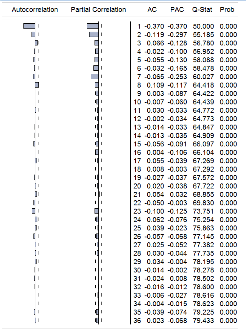
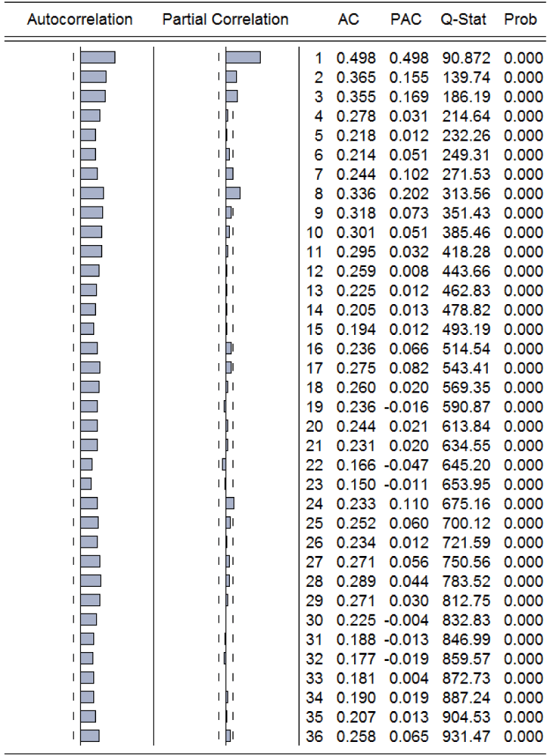
A correlogram is a visual diagnosis for the stationary test. For example, Table 1a is the solar irradiance series correlogram for data from the Green platform. In the autocorrelation column, spikes are outside the two lines indicating no stationarity. Moreover, the Q-stat was given as in 1:

Table 1a: Solar irradiance series correlogram for data from the Green platform.

$Q=T(T+2){\displaystyle \sum _{k=1}^m\frac{{\widehat{\rho }}_k^2}{T-K}}\text{ (1)}$

Where k is the number of lags, T is the total number of observations, m is the lag length, and ${\widehat{\rho }}_k$ is the estimated values at lag k. Table 1b is the first difference solar correlogram. Similar diagrams have been obtained respectively for power output and module temperature but are not indicated here. Table 1b, indicates that stationary series is obtained for the first difference and the EG principle should be applied at a level as indicated below.

Table 1b: Stationary series is obtained for first difference and the EG principle should be applied.

Engle & granger model

The EG test for cointegration is a three-step procedure.

First step: it is necessary to ensure that the first differences of the corresponding Z_t and X_t series are stationary series and where Z_t is regressed on X_t.

Second step: let e_t be the residual of the regression of Z_t with respect to X_t given as follows:

Z_t = aX_t + b + e_t (2)

and if e_t is stationary then Z_t and X_t series are cointegrated and the relationship is usually called long-run equilibrium.

Third step: Error Correction Model (ECM) to reconcile the short-run behavior with long-run behavior.

We applied the first and second steps and computed the regression as each variable is stationary in difference and the resulting equation is given as follows :

$\Delta P=0.969\Delta G+0.500\Delta T-0.105\text{ (3)}$

From the resulting table of the regression difference data, we noted that the corresponding p - value of ∆T and constant term C are not statistically significant because their corresponding probability value (0.4077, 0.9953) are greater than the usual significance level of 1%, 5%, and 10%.

$\Delta P=0.969\Delta G\text{ (4)}$

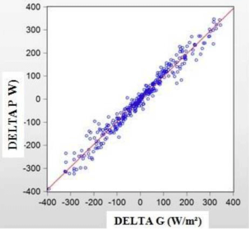
We thus removed ∆T and 0.105. The R2 value is more than 94%. The corresponding plot of the ∆P against ∆G is illustrated in Figure 1.

Figure 1: Regression of ∆P against ∆G.

From Figure 1, we deduced that scattered values and the slight intercept at ∆P axis are indications of heteroscedasticity [14]. We, therefore, applied the Goldfeld quant test followed by the Durbin Watson D-Stat test but the regression model was still not appropriate and we deduced that the ECM must be applied.

The ECM which is the third step of the EG model is applied to equation 2 and is given as follows:

$\Delta P={\alpha }_0+\alpha \Delta G+\beta e_{t-1}+{\epsilon }_t\text{ (5)}$

Where ∆ is the first difference operator, εt is a random error term, e_t-1 is the equilibrium error term, and if β contains a negative sign meaning that a run long equilibrium exists among the variables. After computing, the characteristic terms of the ECM regression without the constant term are illustrated in Table 2.

The Residcoint(-1) is the e_t-1 value with a negative sign validating the long-run relationship between P and G . The final relationship between variables is deduced from Table 2.

$\Delta P=0.966\Delta G-0.601e_{t-1}\text{ (6)}$

Discussion

For the EG statistical method, we investigated the dependent variable P on explanatory variables such as G and T and showed that the first difference of P is a function of only solar irradiance at the level. We showed that the model equation is in agreement with experimental measurements. However, when more explanatory variables are considered the EG is no longer suitable and another model such as the Johansen VECM cointegration model must be applied. This is discussed in the next section.

Johansen VECM cointegration

In this section, we are considering the Johansen VECM cointegration applied to data from a grid-connected PV system on Reunion island in the Indian Ocean. The Johansen VECM cointegration test can be considered a multivariate generalization of the ADF test and makes it possible to estimate all cointegrating vectors when more than two variables are considered.

The Johansen approach

The general form of the VAR (p) model, without drift, is given as in equation 7

$X_t = \pi + A_1 X_{t-1} + \dots \mathrm{..}+ A_p X_{t-p} + {\epsilon }_t\text{ (7)}$

Where π is the vector-valued mean of the series, Ai is the coefficient matrices for each lag, and εt is a multivariate white noise term. The vector error correction model (VECM) is obtained by differencing the series as given in equation 8.

$X_t = \pi + A X_{t-1} + {\gamma }_1 \Delta X_{t-1}\dots \dots \mathrm{..}+ {\gamma }_p \Delta X_{t-p} + {\epsilon }_t\text{ (8)}$

Where ∆X_t = X_t - X_t-1 is the differencing operator, A is the coefficient matrix for the first lag, and γj are the matrices for each differenced lag. The matrix rank is respectively, X_t (N,1), A (N, N), and X_{t -1} (N,1)……. Ap (N, N), X_t (N,1), and εt (N,1), where N is the number of variables of nonstationary I(1). When matrix A = 0 there is no cointegration but for multiple linear combinations of time series the eigenvalue decomposition of A is carried out.

This first difference VAR (2) model can be written in a vector error correction model (VECM) as a function of only Pt-1 as in equation 9:

$\Delta X_t = -A_2 \Delta X_{t-1} + \text{Π} X_{t-1} + {\epsilon }_t\text{ (9)}$

Where $\Pi =A_1+A_2–I$ and I is the unit matrix. Equation 9 can also be written as a function of Pt-1 and Pt-2 as given in Eq.10.

$\Delta P_t = \left(A_1-I\right)\Delta X_{t-1} + \text{Π} X_{t-2} + {\epsilon }_t\text{ (10)}$

If the coefficient matrix Π has reduced rank r < k, where k is the vector variables of I (1), r is the number of cointegration equations. The matrix Π can be written in terms of a vector of adjustment parameters α and a matrix of cointegration vectorsβ’ given by equation 11.

$\Pi =\alpha {\beta }^{\text{'}},\text{ where }{\beta }^{\text{'}}{P}_t\text{ is }I\left(0\right)\text{ (11)}$

Where α is an (N,r) matrix with r < N, and β’ has r cointegration vectors such that 0 < r < N as to highlight the VECM model.

The Johansen test and estimation strategy which is a maximum likelihood test make it possible to estimate all cointegrating vectors for N variables, which all have unit roots and there are at most N-1cointegrating vectors. The Johansen test provides estimates of all cointegrating vectors if a cointegration relationship does exist, and a rank test is useful. Thereby, if:

Rank (Π) = 0, then r = 0 meaning that none cointegration relationship and VECM cannot be applied,

Rank (Π) = r, meaning that variables are cointegrated and the number of cointegration relationships is equal to r. VECM model can be estimated.

Rank (Π) = N, meaning that none cointegration relationship.

Johansen's procedure is based on the maximum Eigenvalue and Trace tests that are conducted on the error correction model foundation. For both test statistics, the initial Johansen test is a null hypothesis test of no cointegration against the alternative of cointegration.

The first test of maximum Eigenvalues is to determine whether the rank of the matrix is zero, and the null hypothesis is rank (Π) = 0 whereas the alternative hypothesis is rank (Π) = 1.

The second test of Trace is to determine whether the rank of the matrix is r0, the null hypothesis is rank (Π) = r0 and the alternative hypothesis is that r0 < rank (Π) ≤ r, where r is the maximum number of possible cointegration vectors.

For the VECM model in this study, variables such as wind speed(Wind), and humidity (Humi) are two more explanatory variables in addition to G & T in the EG section and noted respectively as Irra and Temp in this section. Different forecasting classifications have been proposed and in our study, we should consider the short-term forecast, that is hourly, several hours up to a day ahead to guarantee system commitment and scheduling.

The Johansen VECM test for cointegration is a five-step procedure.

- Step 1: Performing series stationarity (correlogram & ADF) tests to determine whether there is a cointegration relationship or not.

- Step 2: If the step1 is true, meaning that series are of the same order of integration and cointegration is likely, therefore VECM model can be estimated. Determining the lag length using Akaike and Schwarz criteria [3,15].

- Step 3: Implementing the Johansen test to determine the number of cointegration relationships.

- Step 4: Identifying the cointegration relationships or long-term relationships between variables.

- Step 5: Estimating the VECM model by maximum likelihood method, test validations by visual diagnostic or correlogram, and checking that residuals from the model are white noise.

A vector autoregression Pt of 5 variables lagged 2 is given in equation 12:

$P_t=A_1{P}_{t-1}+A_2{P}_{t-2}+{\epsilon }_t\text{ (12)}$

The matrix form is illustrated as follows :

We computed the different steps up to step 3 where the number of cointegration relationships is based on Trace and Eigenvalues [14,16], tests. For this study, this test is performed with the deterministic trend assumption, that is no intercept or trend in the cointegration equation or VAR test. The result after computing the Johansen VECM test with one lagged indicates four cointegration equations. These are indicated in Tables 3a and table 3b are the error correction coefficients.

With data, respectively from Tables 3a and 3b, we identified the 4 equations as follows :

CoinEq1 = (Power _t-1 – 3521,54 Wind _t-1) (14a)

CoinEq2 = (Irra _t-1 – 189,05) (14b)

CoinEq3 = (Temp _t-1 – 16.52 Wind _t-1) (14c)

CoinEq4 = (Himi _t-1 – 0.289 Wind _t-1) (14d)

The ∆P equation is given as follows :

$\begin{array}{l}\Delta P=-0.738{\text{(Power }}_{\text{t-1}}{\text{ - 3521,54 Wind }}_{\text{t-1}}\text{ )}+\text{2}\text{.764}\left({\text{Irra}}_{\text{t-1}}-189,05\right)+29.004\\ \left(Tem{p}_{t-1}-16.52Win{d}_{t-1}\right)+3493.349\left(Hum{i}_{t-1}-0.289Win{d}_{t-1}\right)+{\epsilon }_{1t}\text{ (15)}\end{array}$

For ∆P = P_t – P_t-1, and as each variable at (t-1) is equal to each variable at t , we deduced the long-term relationship as in equation 16:

$P_t=3.74Irr{a}_t+36.38Tem{p}_t+833.33Win{d}_t+4758.96Hum{i}_t+{\epsilon }_{1t}\text{ (16)}$

To determine the residual of the cointegration equation we performed distinct tests such as the Wald test, the Lagrange multiplier test, the jarque bera statistic and finally the CUSUM test indicating that the residual is a random or white noise process. These tests can be easily understood in literature [3].

In the next section, the model obtained is compared to the measured data.

Comparing Johansen model to PV output in reunion island

The Johansen VECM model is applied to forecast PV power output by comparing the model data to measured data in real outdoor conditions. This was done on a yearly basis from 2013 to 2016 for a PV grid connected system in Reunion Island in the Indian Ocean but in this study, we are putting forward a daily comparison upon one month. This is represented in Figure 2, where the blue (series 2) and green (series 1) colors of the bar chart are respectively measured power output and Johansen model power output for each day of the month of march 2016.

Figure 2: Comparing power daily power output between model and measured data.

The model was also applied for an hourly short-term forecast as illustrated in Figure 3.

Figure 3: Comparing hourly power output between model and measured data.

The orange and blue (series1) colors are respectively the Johansen model power output and measured power output.

Conclusion

Power output from photovoltaic (PV) systems in outdoor conditions are substantially influenced by climatic parameters such as solar irradiance and module temperature. One of the objectives of this paper consisted of applying a statistical method of time series data to identify the most important on-site climatic and environmental parameters that influence PV output variability. It is strongly hard to estimate the impact of PV output variability on the power grid stability unless a good comprehension of the parameters controlling this variability. Many OLS regression models relating to PV variables have been proposed in the literature but most of them had led to spurious results. In this paper, two robust statical models have been used in two French territories. The Engle & Granger statistical method is applied in the European zone and the VECM Johansen method is applied to the tropical zone on Reunion island in the Indian Ocean. In this study, we showed that if only these two parameters are considered in the European zone and mainly in the East of France, then the Engle & Granger method is a rigorous method for the long term-term forecast of PV power output. However, when more explanatory variables such as wind speed and humidity are considered in addition to solar irradiation and temperature, the EG method is unable to distinguish several cointegration relationships. We showed that a more robust technique such as the Johansen VECM cointegration must be applied to the Reunion island and can be an accurate technique for short-term forecast of PV power output. From the perspective side in the future, a Spatio-temporal model using recurrent neural networks with persistent short-term memory (LSTM) should be developed to produce efficient forecasts over the whole Reunion island. The developing methodologies should eventually offer an opportunity to provide additional guarantees to the network manager. If in the future efficient forecasting solutions become widespread, this opportunity should open up the market beyond the current regulatory threshold of 35% renewable energy as expected in Reunion Island. Moreover, the mathematical aspects behind the statistical theories should be computed inline code using Python 3.10 and integrated on an FPGA chip in order to be applied at minute sampling time to make more accurate daily predictions.

1. Coban HH, Rehman A, Mohamed A. Technical and economical investigation of a centralized and decentralized hybrid renewable energy system in cadaado, somalia, processes. 2022; 10(4):667. HTTPS://DOI.ORG/10.3390/PR10040667
2. Coban HH. While covid-19 outbreak affects economies and societies; exploring the energy demand in turkey. year. 2021; 11:126–135. HTTPS://DOI.ORG/10.36222/EJT.894463
3. Engle RF,Granger CWJ. co-integration and error correction: representation, estimation, and testing. essays in econometrics. harvard university press 1987 ; 251–276.
4. Granger CWJ, Weiss AA. Time series analysis of error-correction. karlin s, amemiya t, goodman la, éds. studies in econometrics, time series, and multivariate statistics, academic press. 1983; 255–278.
5. Gujarati DN. Basic of econometric, fourth edition. the mcgraw-hill econometrics, fourth companies. 2004.
6. applied economic time series wiley series in probability and statistics.1995; 420.
7. Hassani H, Yeganegi MR. Sum of squared acf and the ljung–box statistics. Phys a: Stat Mech Appl. 2019; 520: 81–86.
8. Ljung GM. Box Gep on a measure of lack of fit in time series models. Biometrika. 1978; 65:297–303.
9. Ramenah H, Casin P, Ba M, Benne M, Tanougast C. accurate determination of parameters relationship for photovoltaic power output by augmented dickey fuller test and engle granger method, AIMS-energy. 2018; DOI: 10.3934/ENERGY.2018.1.19
10. Johansen S. Statistical analysis of cointegration vectors. J Econ Dyn Control .1988; 12: 231–254.
11. Johansen S. Estimation and hypothesis testing of cointegration vectors in gaussian vector autoregressive models. econometrica. 1991; 59: 1551–1580.
12. Johansen S. Likelihood-based inference in cointegrated vector autoregressive models. new york: Ooxford University Press. 1995.
13. Cornillon PA. Regression theorie & application, springer, 2007.
14. Hamilton JD. Time series analysis. princeton university press. 1994; 767–768.
15. Ramenah H, Tanougast C. Techniques of the green platform for research activities. (IOSR Journal of environmental science 2019. DOI:10.9790/2402-1312023241.
16. Long JS, Ervin LH. Using heteroscedasticity consistent standard errors in the linear regression model. the american statistician. 2000; 54: 217-24.