Research on rolling bearing fault feature extraction based on entropy feature

In large machinery, the most common element we can use is rolling bearing. When the rolling bearing fails, it is very likely to affect the normal operation of the equipment, or even cause danger. Therefore, it is necessary to monitor and diagnose the bearing fault in advance. The most important step in fault diagnosis is feature extraction. This is the research content of this paper. In this paper, the approximate entropy, the sample entropy and the information entropy are analyzed, and the feature is extracted to diagnose the rolling bearing fault. The specific research contents are as follows: (1) Firstly, the concepts of approximate entropy, sample entropy and information entropy are introduced briefly, and the approximate entropy, sample entropy and information entropy of rolling bearing vibration signals under different fault modes are calculated. The feasibility and shortcomings of the features extracted from these three entropy in the fault characteristics of rolling bearing are analyzed. (2) In order to make up for their defects, a method of fault feature extraction based on approximate entropy, sample entropy and information entropy is proposed, and its feasibility is verified. (3) Simulation experiments are carried out to calculate the accuracy of fault feature extraction based on the joint analysis of approximate entropy, sample entropy and information entropy.

Introduction

In various fields of large or small machinery, rolling bearing in which the status is indispensable, can be said to play an important role in production and life. For such an important rolling bearing, its fault diagnosis must be paid attention to. Need to be specific to the rolling element fault, inner ring fault or outer ring fault, so that we can carry out subsequent improvement [1]. If only one standard is used for inspection and maintenance, it will not only have low accuracy, but also consume manpower and material resources. If accurate fault diagnosis can be carried out, prevention first and moderate maintenance can be carried out at the same time to avoid bad effects. It is boundto play a very importantrole in promoting economic and social development.

The methods of mechanical equipment fault diagnosis are generally realized by extracting the characteristic information that can represent the state of the equipment. However, the vibration data collected usually contains complex environmental noise and other interferences, which leads to the failure of accurate detection of mechanical equipment by the general time-frequency analysis method [2]. Rolling bearing is an important part of mechanical equipment, its safe operation is related to the operation of the whole equipment, so the accurate diagnosis of bearing fault becomes extremely important.

The research of rolling bearing fault diagnosis began around 1960. On the whole, it can be divided into five stages.The first stage is spectrum analysis in 1950s. The method of spectrum analysis has attracted much attention. However, due to the immature technology at that time, spectrum analysis has not been widely used in the field of bearing fault diagnosis technology because of the disadvantages of interference noise, high price and complex operation.

In the second stage, in the sixties of the 20th century, the impact pulse meter detection method appeared, which is obviously better than the spectrum analysis, and can directly save the complicated steps. It is still widely used in the fault diagnosis of rolling bearing. In the third stage, in the 1960s1980s, the computer and signal have made great progress under the promotion of the trend of the times, and the more prominent one is the resonance demodulation technology, because the advent of this technologymakes the rolling bearing fault diagnosis technology to a higher level, from birth to maturity step by step [3].

The fourth stage is after the 1980s, the emergence of artificial intelligence provides new soil for rolling bearing fault diagnosis, and the emergence of intelligent diagnosis system greatly improves the accuracy of fault diagnosis. Due to the intelligence, the influence of human factors is greatly reduced, which has been applied in engineering practice.In order to enable nonsignal analysis specialists to monitor the running state and reduce the engineering cost as much as possible, Janssens proposed a learning model based on convolutional neural network, which learned the function of detecting bearing faults from the vibration signal itself. In view of the nonlinearity and non-stability of the vibration signal of rolling bearing, Ben proposed the mathematical analysis of selecting the most importantintrinsic mode functionby combining the method of extracting energy entropy by empirical mode decomposition. The fifth stage is after the 21st century, that is, we now, rolling bearing fault diagnosis technology has taken an epoch-making step, more and more high-tech development, through the virtual instrument fault diagnosis, has become a new beacon, has important practical value [4]. At present, rolling bearing fault diagnosis has been studied all over the world, combining a large number of different research fields. According to the most popular classification method, it can be divided into three kinds, which are modelbased fault diagnosis technology, knowledge-based fault diagnosis technology and data-based fault diagnosis technology.

Because of the national conditions, our country started to study the fault diagnosis much later than other countries. It was not until the late 1970s and the early 1980s that I first came into contact with this field and started formal research. But it is gratifying that with the hard work of Chinese researchers, in the 1990s, the field of fault research has been on the right track, both in theory and practice have made great breakthroughs, and can be applied in production and life. But compared with other countries, China still has a long way to go.

Scheme design

Approximate entropy

Approximate Entropy (ApEn) is a nonlinear dynamic parameter proposed by Pincus in 1991 to measure the complexity and statistical quantification of a sequence. ApEn reflects the degree of self similarity of sequence in pattern. The higher the ApEn value is, the lower the possibility that the system can predict it. It gives the situation that the incidence of new pattern increases or decreases with the dimension, so as to reflect the complexity of data structure. Through the previous, we can know that rolling bearing will produce vibration, and in different failure modes, the vibration signal is also different. According to the physical meaning of ApEn, different signals mean different complexity, which can be used as features for rolling bearing fault diagnosis [5].

In the normal calculation of approximate entropy, there are too many redundant calculations, which is a waste of time. A fast algorithm of approximate entropy is given in the literature.

Let the original sequencebe u(i),i=0,1,,N,r=0.10.25SD(u) (SD is the standard deviation of sequence u(i)), then the calculation of approximate entropy is more reasonable. If m = 2, then N = 5001000.3.

Calculate the distance matrix d of N×N, and the elements in row I and column j of d are written as d_ij

$d_{ij}=\{\begin{array}{c}1 \left|u\left(i\right)-u(j)\right|<r\\ 0 \left|u\left(i\right)-u(j)\right|\ge r\end{array}$ (1)

Use that elements in d, calculate $C_i^2(r),C_i^3(r)$

$C_i^2\left(r\right)={\displaystyle \sum }_{j=1}^{N-1}{d}_{ij}{{\displaystyle \cap }}^{\text{}}{d}_{(i+1)(j+1)}$ (2)

$C_i^3(r)={\displaystyle \sum }_{j=1}^{N-2}{d}_{ij}{{\displaystyle \cap }}^{\text{}}{d}_{(i+1)(j+1)}{{\displaystyle \cap }}^{\text{}}{d}_{(i+1)(j+2)}$ (3)

$\text{ApEn}\left(\text{m},\text{r},\text{N}\right)=H^n(r)-H^{n+1}(r)$ (4)

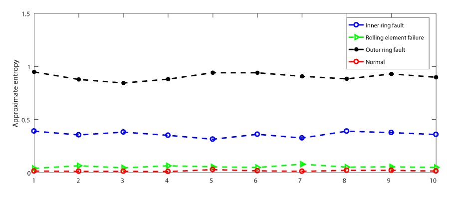
Take out the first 6000 data and calculate the approximate entropy in a group of 600, as shown in Figure 1.

Figure 1: Approximate entropy curve

It is not difficult to see that when the rolling bearing is normal, the value of approximate entropy is not large, because under normal conditions, the signal generated is relatively single. When the rolling bearing fails, it will produce a lot of complex information, which will increase the approximate entropy. However, the approximate entropy values of rolling element fault and normal working conditions are very similar, so it is not easy to distinguish them.

Sample entropy

In 2000, Richman, et al. First proposed the concept of sample entropy, which is a more robust time series complexitymeasurementmethodsimilar to approximateentropy. Compared with approximate entropy, it has stronger antiinterference and anti noise ability [7]. Sample entropy improves the algorithm of approximate entropy, which can reduce the error of approximate entropy. It is similar to approximate entropy, but its accuracy is better [6].

Sample entropy is a new measure of time series complexity proposed by Richman and moornan. The improvement of the sample entropy algorithm compared with the approximate entropy algorithm: compared with the approximate entropy, the sample entropy calculates the logarithm of sum. The purpose of sample entropy is to reduce the error of approximate entropy, which is more consistent with the known random part. Sample entropy is similar to the present approximate entropy but has better accuracy. Compared with approximate entropy, sample entropy has two advantages: first, sample entropy does not include the comparison of its own data segments, it is the exact value of negative average natural logarithm of conditional probability, so the calculation of sample entropy does not depend on the data length; Second, sample entropy has better consistency. That is, if one time series has a higher value than another time series, it also has a higher value for other m and R values.

Assume that the data is $\left\{X_i\right\}=\{x_{1,}{x}_2,\dots ,x_N\}$ , and its length is n, and then reconstruct an m-dimensional vector from the original signal $x_i=[x_i,x_{i+1},\dots ,x_{i+m-1}]$

Define the distance between A and B

$d_{ij}=d\left[x\left(i\right),x\left(j\right)\right]=\underset{k\in [0,m-1]}{\max }[\left|x\left(i+k\right)-x(j+k)\right|]$ (5)

Count the number of dij less than the similarity tolerance r and the ratio of the number to the total number of d_ij N-m-1, and record it as

$B_i^m\left(r\right)=\frac{1}{N-m-1}$ (6)

$SampEn(m,r,N)=\ln B^m\left(r\right)-\ln B^{m+1}\left(r\right)$ (7)

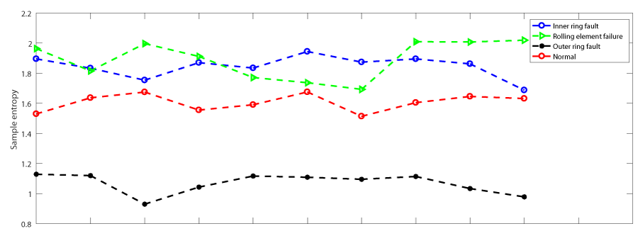
Take the first 6000 data, take 600 as a group, and calculate the sample entropy, as shown in Figure 2.

Figure 2: Sample entropy curve.

It is not difficult to see that the inner ring fault, rolling element fault and normal working conditions are very difficult to distinguish, but the outer ring fault can be distinguished.

Information entropy

Claude E. Shannon, one of the originators of information theory, defined information (entropy) as the probability of occurrence of discrete random events.

X represents a random variable, the value of which is $(x1,x2,\mathrm{...}xn)$ and p(xi) represents the probability of occurrence of event xi.

$H\left(X\right)=-{{\displaystyle \sum }}^{\text{}}p\left(xi\right)\log \left(p\left(xi\right)\right) (i=1,2,\dots ,n)$ (8)

The so-called information entropy is a very abstract concept in mathematics. Here we might as well understand information entropy as the probability of certain information. Information entropy and thermodynamic entropy are closely related. According to Charles h. Bennett’s reinterpretation of Maxwell’s demon, the destruction of information is an irreversible process, so the destruction of information conforms to the second law of thermodynamics. The generation of information is the process of introducing negative entropy into the system. So the sign of information entropy and thermodynamic entropy should be opposite.

Generally speaking, when a kind of information has a higher probability of occurrence, it means that it has been spread more widely, or that it has been cited to a higher degree. We can think that from the perspective of information dissemination, information entropy can express the value of information. In this way, we have a standard to measure the value of information, and we can make more inferences about knowledge flow.

Take the first 6000 data and calculate the information entropy in a group of 600, as shown in Figure 3.

Figure 3: Sample entropy curve

We can see that the rolling element fault and the normal working condition intersect, and the inner ring fault and the outer ring fault are also very close to each other. If the information entropy is not processed, it is difficult to distinguish the rolling element fault and the normal working condition, and it is easy to misjudge the inner ring fault and the outer ring fault.

Three entropy joint analysis

Three kinds of entropy in the case of independent judgment have no small disadvantages, it is easy to misjudge the situation, need to be further processed. So I started to study the extraction of rolling bearing fault features through the joint analysis of approximate entropy, sample entropy and information entropy.

• The original vibration signals of rolling bearing under normal working condition and different fault types are collected, and 100 groups of sample data under each working condition are selected.

• The approximate entropy, sample entropy, information entropy and average value are calculated.

• The entropy characteristic scale of fault extraction of rolling bearing is obtained.

• The original vibration signals of rolling bearing under normal working condition and different fault types are collected, and 10 groups of sample data under each working condition are selected.

• The approximate entropy, sample entropy and information entropy of ten groups of data are calculated.

• Compared with the extracted entropy feature.

• According to the absolute value of the difference with the entropy characteristic scale, which bearing working state is closest to the test data can be judged.

Simulation experiment

Data source: The data used in this paper are all from the bearing data center of Case Western Reserve University. The model of experimental bearing is 6205-2RS JEM SKF deep grooveball bearing.

The acceleration vibration sensor placed on the driving end of the bearing is used to collect the vibration acceleration signal. It uses electric spark technology to damage the rolling body, inner ring and outer ring of the bearing. The damage diameter is 0.1778 mm, 0.3556 mm and 0.5334 mm. The fault diameter selected in this paper is 0.1778 mm. The data used in this paper is divided into normal working condition, ball fault, outer ring fault and inner ring fault. The sampling frequency is 12Khz and the motor speed is 1750r/min.

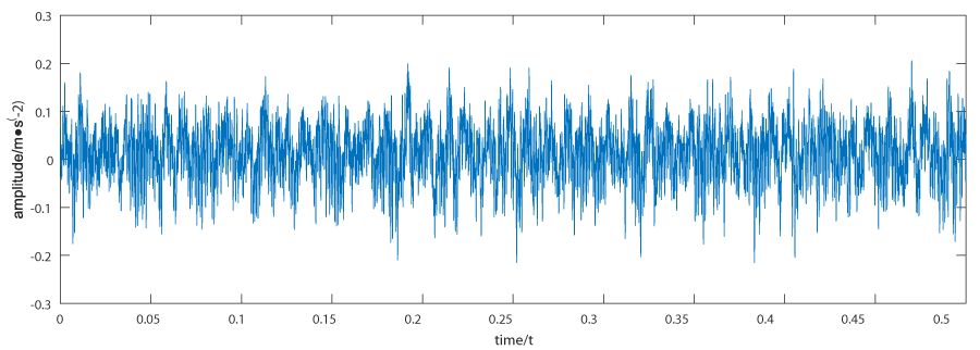
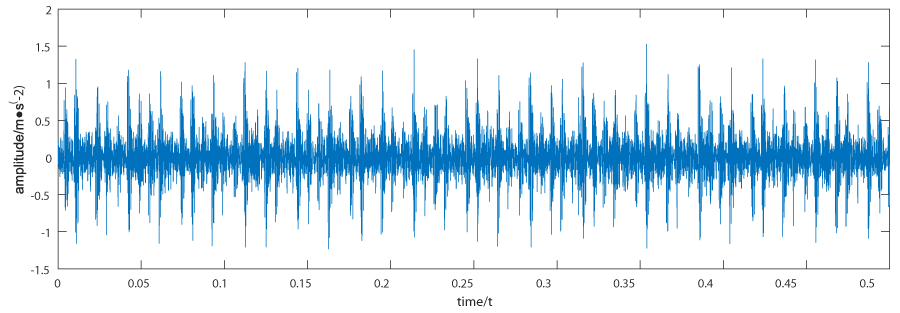
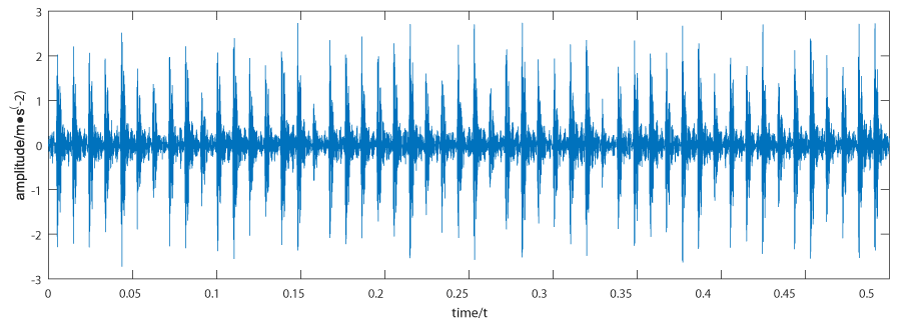
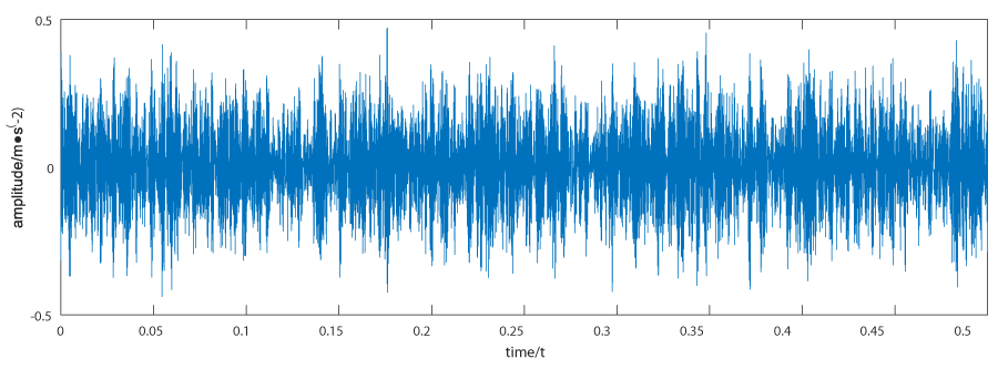
Specific implementation mode: In the first step, collect the original signals of normal working conditions and different fault states of rolling bearing. The total data amount of each working condition is 120000. Then, 10 groups of sample data for each working condition are selected, and the data volume of each group is 6000. The time-domain image of the first group of sample data is shown in Figures 4-7.

Figure 4: Normal bearing signal.

Figure 5: Inner ring fault signal.

Figure 6: Outer ring fault signal.

Figure 7: Rolling element fault signal.

Three kinds of entropy in the case of independent judgment have no small disadvantages, it is easy to misjudge the situation, need to be further processed. So I started to study the extraction of rolling bearing fault features through the joint analysis of approximate entropy, sample entropy and information entropy. The data is taken from the Western Reserve University. Under the working condition of 2 HP load, 0.1778 mm fault diameter and 1750 R / min rotating speed, the vibration acceleration signals under four different modes are obtained. There are four groups corresponding to different modes, with 60000 data in each group. Each group is divided into 10 sections, with 6000 data in each section. Each section is divided into 10 sections, with 600 data in each section Each section calculates an approximate entropy, sample entropy and information entropy, and each group has ten entropy values to do mean processing, which can get ten approximate entropy mean values, sample entropy mean values, and information entropy mean values of each section. shown in Figures 8-10.

Figure 8: Approximate entropy mean.

Figure 9: Sample entropy mean.

Figure 10: Mean value of information entropy.

As can be seen from Fig, for each fault mode, there are two kinds of entropy features that can be distinguished. As long as the features of the three kinds of entropy mean in each fault mode are extracted, four groups of column vectors are formed, as shown in Table 1, each column corresponds to the entropy feature vector under the working condition.

Then, the same entropy characteristic column vectors obtained from the same four test data are used to form the test data entropy characteristic matrix.

Taking the average entropy feature vector as the benchmark, we compareit with the test data entropyfeature vector, that is, take the absolute value after the difference, and get four new vectors. The four new vectors are combined into an entropy characteristic matrix, and the minimum value of each row in the matrix is taken out. The maximum number of columns corresponding to the minimum value is the closest test data to the fault mode. However, in rare cases, three kinds of entropy features will judge three kinds of fault modes. At this time, the fault mode corresponding to the maximum discrimination approximate entropy mean value will be taken as the final fault mode of test data.

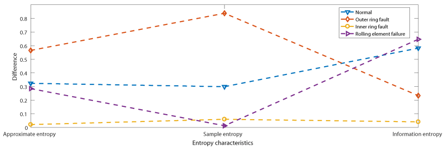
After the early stage of rolling bearing fault feature extraction, we have extracted the approximate entropy mean value, sample entropy mean value and information entropy mean value of four rolling bearing fault modes. By comparing the feature vectors, we can effectively distinguish the four fault modes. A 6000 data matrix is randomly generated by using the data, and the fault feature of the matrix is extracted, and the fault condition is determined. Then the results are compared with the previously established standard, and each group is tested 500 times, at least 10 groups are done to test its accuracy. Based on the above description, the simulation experiment is started. It is also taken from the Western Reserve University. Under the working condition of 2 HP load, 0.1778 mm fault diameter and 1750 R/ min rotating speed, the vibration acceleration signals under four different modes are obtained. From the last 60000 data, 6000 outer ring fault data are divided into ten sections, each section has 600 data, and approximate entropy, sample entropy and fuzzy entropy mean are calculated to form column vector in Figure 11.

Figure 11: Entropy characteristic difference 1.

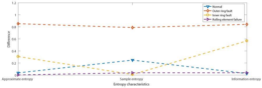
If the difference between the mean approximate entropy and the mean information entropy of the inner ring fault is the smallest, it is judged that the test data is the inner ring fault mode. The same is true for other failure modes. The test vector in the test data is extracted, which is different from the entropyeigenvector,and the minorityis subordinate to the majority. This paper focuses on the special case. The difference between the feature vector and the test vector is selected in the case of rolling element failure in Figure 12, Table 2.

Figure 12: Entropy characteristic difference 2.

It can be seen that the approximate entropy feature gets the minimum value in rolling element fault, the sample entropy feature gets the minimum value in inner ring fault, and the information entropy feature gets the minimum value in normal condition. At this time, we select the condition corresponding to the approximate entropy feature as the final result.

Conclusion

Based on approximate entropy, sample entropy and information entropy, a joint diagnosis method for rolling bearing fault is proposed.

According to the characteristics of entropy signal, fault diagnosis is carried out. The experimental results show that the accuracy of the three entropy joint fault diagnosis methods is more than ninety-seven percent. And it can correctly identify each bearing state, which verifies the effectiveness of the fault diagnosis method 2.

1. Cheng D (2005) Controllability of switched bilinear systems. IEEE Trans Automatic Control 50: 511-515. Link: https://bit.ly/3g6Cgbf
2. Ding XX, He QB (2016) Time-frequency manifold sparse reconstruction:A novel method for bearing fault feature extraction. Mechanical Systems and Signal Processing 80: 392-413. Link: https://bit.ly/3AKSjUi
3. Poor H (1985) An Introduction to Signal Detection and Estimation. New York: Springer-Verlag, chapter 4. Link: https://bit.ly/3y0rR7r
4. Smith B (2016) An approach to graphs of linear forms, accepted. Link: https://bit.ly/3ySi987
5. Cheng D (2005) On logic-based intelligent systems. In Proceedings of 5th International Conference on Control and Automation 71–75. Link: https://bit.ly/37S4WAd
6. Cheng D, Ortega R, Panteley E (2005) On port controlled hamiltonian systems, in Advanced Robust and Adaptive Control — Theory and Applications. In D Cheng, Y Sun, T Shen and H Ohmori, Eds. Beijing: Tsinghua University Press 2005: 3–16.