Mid-point technique for calculating divergent integrals

A mid-point technique is introduced to overcome the difficulties in other techniques. The modied e⁄ective interaction quark potential which uses to calculate different properties of the NJL model such as the constituent quark mass, pressure, and energy density is solved using the present technique. The present method gives good accuracy for the mathematical problem and avoids the physical di¢ culty in the previous works.

Introduction

The appearance of divergent integrals in the different mathematical-phyiscal models is a real problem. This problem represents that the treatment of divergence integrals did not give a unique value for divergent integrals such as [1]. There are different methods for dealing with the divergent integrals such as analytic continuation [2], by regularization [3], by summability methods [4], and by nite part integrals [5,6], and others [7,8]. In these methods, the missing terms have appeared so that no interpretation gives exact results.

In this work, we focus on the quark models that deal with strong interactions between quarks inside nucleon. There are different quark models such as the quark sigma model and its extension [9-15] and Nambu and Jona-Lasinio model (NJL) its extension [16-19]. The NJL is taken as a model for the divergent integral [16]. The NJL model has the divergent integral that obtained from Dirac sea to overcome on this problem, Pauli-Villars and the three-momentum cutoff methods are applied such as [20,21].

Therefore, the N-midpoint technique is applied for treatment the divergence integrals in NJL. In addition, the thermodynamic properties are calculated in the framework of NJL model, in which the coupling constant is generalized as a function of temperature and chemical potential, that is not considered in Ref [19].

The paper is arranged as follows: In Sec. 2, the NJL model is briey written. Sec. 3, thermodynamic properties. are calculated. Sec. 4, the discussion of results is explained.

The nambu-jona-lasinio model

The interactions between quarks (q) via scalar qq and pseudoscalar q₅ q [18], in the framework of NJL model is given through the Lagrangian density is,

$L\left(x\right)\mathrm{<mo>=</mo>}\overline{q}\mathrm{<mo\; stretchy="false">(</mo>}i{\partial }_{\mu }{\gamma }^{\mu }-m_0\mathrm{<mo\; stretchy="false">)</mo>}q+\frac{G_0}{2}\left({\mathrm{<mo\; stretchy="false">(</mo>}\overline{q}q\mathrm{<mo\; stretchy="false">)</mo>}}^2+{\mathrm{<mo\; stretchy="false">(</mo>}\overline{q}{\gamma }_5\tau q\mathrm{<mo\; stretchy="false">)</mo>}}^2\right)\mathrm{,}\text{ (1)}$

sm₀ is the bare quark mass. The are the Pauli matrices. The NJL Lagrangian satised the chiral symmetry property at m₀ = 0. In the present work, the coupling constant G is extended to nite temperature (T)and chemical potential ( ) as follows

$G\left(T\mathrm{,}\mu \right)\mathrm{<mo>=</mo>}{G}_0{e}^{-A\left(T+\mu \right)}\text{ (2)}$

where, A is a free parameter in MeV ¹ units. The G(T;) tends to G₀ at T = 0 and = 0

The Used Method

The N-midpoint technique is used to calculate the thermodynamic properties. The scalar density is written as in Ref. [18].

${\rho }_s\mathrm{<mo>=</mo>}\langle \overline{q}q\rangle \mathrm{<mo>=</mo>}\frac{6M}{{\pi }^2}{\displaystyle {\int }_0^{\infty }}\frac{1}{\sqrt{p^2+M^2}}\left(n_q\left(T\mathrm{,}\mu \right)+n_{\overline{q}}\left(T\mathrm{,}\mu \right)-1\right)p^{2}dp\mathrm{.}\text{ (3)}$

The dimensionless form of Eq. (3) is obtained as follows

${\rho }_s\mathrm{<mo>=</mo>}\langle \overline{q}q\rangle \mathrm{<mo>=</mo>}{\frac{6M}{{\pi }^2}}^{\text{'}}{\displaystyle {\int }_0^{\infty }}\frac{\left(n_q\left(T^{\text{'}}\mathrm{,}{\mu }^{\text{'}}\right)+n_{\overline{q}}\left(T^{\text{'}}\mathrm{,}{\mu }^{\text{'}}\right)-1\right)}{\sqrt{p^{\text{'}2}+M^{\text{'}2}}}{p}^{{}^{\text{'}}2}d{p}^{\text{'}}\mathrm{,}\text{ (4)}$

Where

$p^{\text{'}}\mathrm{<mo>=</mo>}\frac{p}{f_{\pi }}\mathrm{,}{T}^{\text{'}}\mathrm{<mo>=</mo>}\frac{T}{f_{\pi }}\mathrm{,}{M}^{\text{'}}\mathrm{<mo>=</mo>}\frac{M}{f_{\pi }}\text{,and}{\mu }^{\text{'}}\mathrm{<mo>=</mo>}\frac{\mu }{f_{\pi }}\mathrm{.},\text{ and} { }^0=\text{ (5)}$

f = 93 MeV is pion decay constant. The third term in Eq. (3) is a divergent term. To apply the mid-point method, the formula y = e ^p0 is used at fy = 1 at p0 = 0 and y = 0 at p0 = 1g. Therefore, s is calculated as a function of y as follows:

${\rho }_s\mathrm{<mo>=</mo>}{\frac{6M}{{\pi }^2}}^{\text{'}}{\displaystyle {\int }_0^1}\frac{\left(n_q\left(T^{\text{'}}\mathrm{,}{\mu }^{\text{'}}\right)+n_{\overline{q}}\left(T^{\text{'}}\mathrm{,}{\mu }^{\text{'}}\right)-1\right)}{y\sqrt{{{\displaystyle \ln }}^{2}y+M^{{}^{\text{'}}2}}}{{\displaystyle \ln }}^{2}ydy\mathrm{,}\text{ (6)}$

Where

$n_q\left(T^{\text{'}}\mathrm{,}{\mu }^{\text{'}}\right)\mathrm{<mo>=</mo>}\frac{1}{1+\exp \mathrm{<mo\; stretchy="false">[</mo>}\frac{\mathrm{<mo\; stretchy="false">(</mo>}\sqrt{{{\displaystyle \ln }}^{2}y+M^{{}^{\text{'}}2}}-{\mu }^{\text{'}}\mathrm{<mo\; stretchy="false">)</mo>}}{T^{\text{'}}}\mathrm{<mo\; stretchy="false">]</mo>}}\mathrm{,}{n}_{\overline{q}}\left(T^{\text{'}}\mathrm{,}{\mu }^{\text{'}}\right)\mathrm{<mo>=</mo>}{n}_q\left(T^{\text{'}}\mathrm{,}-{\mu }^{\text{'}}\right)\mathrm{.}\text{ (7)}$

The analytic function of s is calculated by using the N-midpoint method as in Ref. [23], as follows:

$\begin{array}{l}{\rho }_s\mathrm{<mo>=</mo>}\frac{6M^{\text{'}}}{n{\pi }^2}{\displaystyle \sum _{i\mathrm{<mo>=</mo>0}}^{n-1}}\frac{{{\displaystyle \ln }}^2\left(A_i\right)}{A_i\sqrt{M^{{}^{\text{'}}2}+{{\displaystyle \ln }}^2\left(A_i\right)}}\mathrm{<mo\; stretchy="false">[</mo>}\frac{1}{\exp \left(\frac{1}{T^{\text{'}}}\left({\mu }^{\text{'}}+\sqrt{M^{{}^{\text{'}}2}+{{\displaystyle \ln }}^2\left(A_i\right)}\right)\right)+1}+\\ +\frac{1}{\exp \left(\frac{1}{T^{\text{'}}}\left(\sqrt{M^{{}^{\text{'}}2}+{{\displaystyle \ln }}^2\left(A_i\right)}-{\mu }^{\text{'}}\right)\right)+1}-\mathrm{1<mo\; stretchy="false">]</mo>,}\text{ (8)}\end{array}$

where Ai is dened as follows:

$A_i\mathrm{<mo>=</mo>}\frac{1}{n}i+\frac{1}{2n}\mathrm{.}\sqrt{b^2-4ac}\text{ (9)}$

Similarly, the thermodynamic potential is written as a function of variable y using y = e ^p0

$\begin{array}{l}\Omega \mathrm{<mo>=</mo>}\frac{{\left(M^{\text{'}}-m_0^{\text{'}}\right)}^2}{2G^{\text{'}}}-\frac{6}{{\pi }^2}{\displaystyle {\int }_0^1}\frac{{{\displaystyle \ln }}^{2}y}{y}dy\mathrm{<mo>\{</mo>}\sqrt{{{\displaystyle \ln }}^{2}y+M^{{}^{\text{'}}2}}+\\ T{\mathrm{<mi>\; </mi>}}^{\text{'}}\ln \mathrm{<mo\; stretchy="false">[</mo>1}+\exp \left(-\frac{\sqrt{{{\displaystyle \ln }}^{2}y+M^{{}^{\text{'}}2}}+{\mu }^{\text{'}}\mathrm{<mo\; stretchy="false">)</mo>}}{T^{\text{'}}}\right)\mathrm{<mo\; stretchy="false">]</mo>}+\\ +T{\mathrm{<mi>\; </mi>}}^{\text{'}}\ln \mathrm{<mo\; stretchy="false">[</mo>1}+\exp \left(-\frac{\mathrm{<mo\; stretchy="false">(</mo>}\sqrt{{{\displaystyle \ln }}^{2}y+M^{{}^{\text{'}}2}}-{\mu }^{\text{'}}\mathrm{<mo\; stretchy="false">)</mo>}}{T^{\text{'}}}\right)\mathrm{<mo\; stretchy="false">]</mo><mo>\}</mo>,}\text{ (}10)\end{array}$

Where

$m_0^{\text{'}}\mathrm{<mo>=</mo>}\frac{m_0}{f_{\pi }}\text{and}{G}^{\text{'}}\mathrm{<mo>=</mo>}G\mathrm{<mi>\; </mi>}{f}_{\pi }^2\mathrm{.}\text{ (11)}$

The analytic form of is

$\begin{array}{l}\Omega \mathrm{<mo\; stretchy="false">(</mo>}{T}^{\text{'}}\mathrm{,}{\mu }^{\text{'}}\mathrm{<mo\; stretchy="false">)</mo><mo>=</mo>}\frac{{\left(M^{\text{'}}-m_0^{\text{'}}\right)}^2}{2G^{\text{'}}}-\frac{6}{n{\pi }^2}{\displaystyle \sum _{i\mathrm{<mo>=</mo>0}}^{n-1}}\frac{1}{A_i}\left({{\displaystyle \ln }}^2\left(A_i\right)\right)\mathrm{<mo\; stretchy="false">(</mo>}\sqrt{M^{\text{'}2}+{{\displaystyle \ln }}^2\left(A_i\right)}+\\ \\ T^{\text{'}}\ln \left(\exp \left(-\frac{1}{T^{\text{'}}}\left({\mu }^{\text{'}}+\sqrt{M^{{}^{\text{'}}2}+{{\displaystyle \ln }}^2\left(A_i\right)}\right)\right)+1\right)+\\ \\ +T^{\text{'}}\ln \left(\exp \left(-\frac{1}{T^{\text{'}}}\left(-{\mu }^{\text{'}}+\sqrt{M^{\text{'}2}+{{\displaystyle \ln }}^2\left(A_i\right)}\right)\right)+1\right)\mathrm{<mo\; stretchy="false">)</mo>.}\text{ (}12)\end{array}$

Also, we can dene the energy density as in Ref. [25], as follows:

$E\mathrm{<mo\; stretchy="false">(</mo>}{T}^{\text{'}}\mathrm{,}{\mu }^{\text{'}}\mathrm{<mo\; stretchy="false">)</mo><mo>=</mo>}-P\mathrm{<mo\; stretchy="false">(</mo>}{T}^{\text{'}}\mathrm{,}{\mu }^{\text{'}}\mathrm{<mo\; stretchy="false">)</mo>}+T^{\text{'}}\frac{\partial P\mathrm{<mo\; stretchy="false">(</mo>}{T}^{\text{'}}\mathrm{,}{\mu }^{\text{'}}\mathrm{<mo\; stretchy="false">)</mo>}}{\partial T^{\text{'}}}+{\mu }^{\text{'}}\frac{\partial P\mathrm{<mo\; stretchy="false">(</mo>}{T}^{\text{'}}\mathrm{,}{\mu }^{\text{'}}\mathrm{<mo\; stretchy="false">)</mo>}}{\partial {\mu }^{\text{'}}}\mathrm{,}\text{ (13)}$

Where

$P\mathrm{<mo\; stretchy="false">(</mo>}{T}^{\text{'}}\mathrm{,}{\mu }^{\text{'}}\mathrm{<mo\; stretchy="false">)</mo><mo>=</mo>}-\Omega \mathrm{<mo\; stretchy="false">(</mo>}{T}^{\text{'}}\mathrm{,}{\mu }^{\text{'}}\mathrm{<mo\; stretchy="false">)</mo>.}\text{ (14)}$

Results and Discussion

In this section, we give the features of the midpoint technique in comparison with other methods. The fewer errors are obtained in comparison with other numerical methods as in Ref. [23]. In comparison with the cutoff technique. Two advantages are found, from the mathematical view, the upper of momentum value depends on to the parameter n, which gives a good accuracy by increasing the parameter n as noted in table (1). Another advantage, by transforming the innite divergence integral to nite divergence, we control in the missing terms that found in other methods. From the physical situation, the color superconductivity is found at the critical chemical potential that is the order of the cutoff parameter. Thus, the regularization procedure has a small e⁄ect on the analysis of the color superconductivity [11].

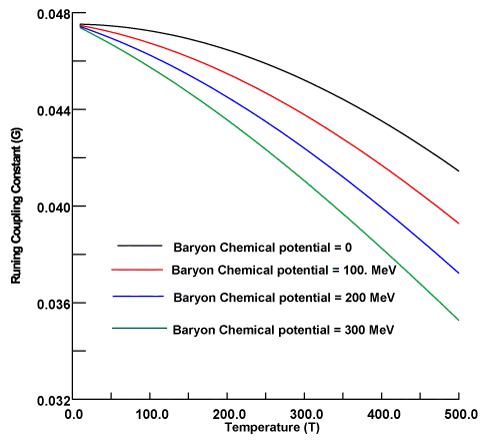
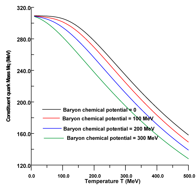
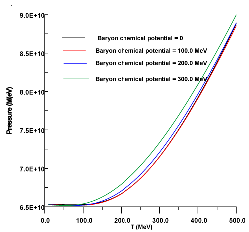
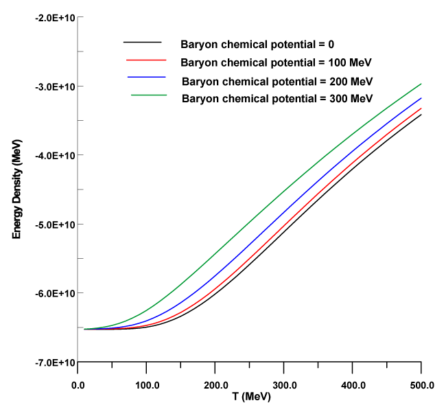
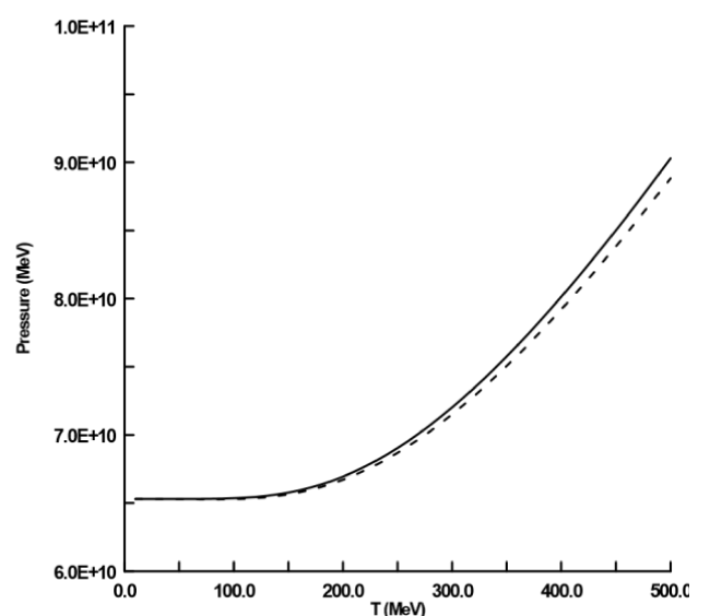
In figure 1, the coupling constant is plotted as a function of temperature by using Eq. (2). At zero temperature and baryon chemical potential, the running coupling constant tends to G0 in the vacuum, then by increasing temperature, one notes that the coupling constant decreases with increasing temperature. In addition, the coupling constant is strongly affected with the baryon chemical potential at higher values of temperatures. By increasing baryon chemical, the running coupling drops to lowers values. In figure 2, the constituent quark mass is plotted as a function temperature. One notes that the constituent quark mass is steady function up to 75 MeV, then the constituent quark mass decreases with increasing temperature at zero chemical potential. By increasing chemical potential, the constituent quark mass drops to lower values. In comparison with Refs. [18,19], the behavior of constituent quark mass is the qualitative agreement with the results of Refs. [18,19], in which the running coupling is not considered. In figures 3,4 the pressure is plotted as a function of temperature. One notes that the pressure is increasing function with temperature and shifts to higher values by increasing baryon chemical potential. Moreover, the pressure is not sensitive up to 100 MeV, then the pressure is a sensitive quantity when baryon chemical potential increases more than 150 MeV. The finding is agreement with the conclusion of Refs. [24,25]. A similar situation for energy density, the energy density increases with increasing temperature and shifts to higher values by increasing baryon chemical potential. In addition, the energy density is steady function up to 75 MeV.

The coupling constant G is plotted as a function of temperature for di⁄erent values of baryon chemical potential.

The constituent quark mass is plotted as a function of temperature for di⁄erent values of baryon chemical potential.

The pressure is plotted as a function temperature for di⁄erent values of baryon potential, of baryon chemical potential.

The energy density is plotted as a of function of temperature for di⁄erent values chemical.

In figures 5,6 the consistent quark mass is plotted in the two cases. In the first case, when the coupling constant is constant and the second case is dependent on temperature and baryon chemical potential. The consistent quark mass drops to lower values at higher values of temperature in the second case. A similar situation, the pressure drops to lower values when the dependent coupling temperature is considered. Therefore, the effect of running coupling constant on the quantitative values of observables which leads to the phase transition is kept as crossover as in Refs. [18,19]

The constitent quark mass is plotted as a function of temperture where the sold curve represents the constant counpling constant and dash curve represents the running coupling constant.

The pressure is plotted as a function of temperture where the sold curve represents the constant counpling constant and dash curve represents the running coupling constant.

Conclusion

In this work, the mid-point method is employed to carry out the divergence integral in the NJL model that found from Dirac sea. To apply this method, the infinite divergence integral to finite divergence integral. Therefore, we avoid the missing terms that found the previous works such as the cut-off technique. In cut-off technique that applied in many works has disadvantages, in which all observables depend on the choice of cutoff parameter. In the present method, the calculated integral depends on the accuracy parameter (n) only. Thus, good accuracy is obtained by controlling in the accuracy parameter (n): The observables such as constituent quark mass, pressure, and energy density are calculated by using the present method with a good accuracy.

The coupling constant is extended to finite temperature and baryon chemical potential. The suggested running coupling constant decreases with increasing temperature and baryon chemical potential. In addition, the running coupling constant tends to the normal coupling constant at zero temperature and baryon chemical potential. All observables are dropped to lower values when the running coupling constant is included. Therefore, the coupling constant is not affected on qualitative behavior of the present observables. This finding is not considered in previous works such as [16-19].