Annals of Limnology and Oceanography
High-frequency modeling of dissolved oxygen and net ecosystem metabolism using STELLA
Miraç Eryiğit*, Fatih Evrendilek and Nusret Karakaya
Cite this as
Eryiğit M, Evrendilek F, Karakaya N (2023) High-frequency modeling of dissolved oxygen and net ecosystem metabolism using STELLA Ann Limnol Oceanogr 8(1): 001-008. DOI: 10.17352/alo.000013Copyright
© 2023 Eryiğit M, et al. This is an open-access article distributed under the terms of the Creative Commons Attribution License, which permits unrestricted use, distribution, and reproduction in any medium, provided the original author and source are credited.This paper proposes a high-frequency process model for estimating Dissolved Oxygen (DO) and net ecosystem metabolism (NEM) in streams. The model was implemented by using STELLA to predict DO concentrations at one-minute intervals downstream of a 150-m headwater reach of the Abant Creek (Bolu, Turkey). NEM was also predicted at each interval by using a two-station method along the reach. DO, water temperature and other environmental variables used in the model were measured during 17 months between August 2015 and December 2016. The model was run for a day representing every month of the year. Model parameters were calibrated and validated according to mean absolute error (MAE) between measured and simulated values of DO and NEM. The results showed that the model appeared to be promising in terms of high-frequency estimations of DO.
Introduction
Dissolved oxygen (DO) is vital for aquatic life. Therefore, DO lack or extreme oscillations of DO affect all creatures living in the water [1-4]. In general, these issues occur due to human activities (discharges, agriculture, etc.) causing variations in DO concentrations shortly [5-9]. Also, natural events such as instantaneous temperature waves, heavy rainfalls and storms may influence DO concentrations in the water [10,11]. Thus, high-frequency DO data are required in order to evaluate sudden reactions of stream and lake ecosystems against extreme events and human activities. In addition, to DO, stream metabolism is also important as one of the fundamental indicators of nutrient, organic matter cycling, and stream health [12-15]. Net ecosystem metabolism (NEM) indicates a heterotrophic or autotrophic situation in streams and other water bodies and is estimated by measuring diurnal variations of DO concentrations due to photosynthesis, respiration, and reaeration [16]. In this regard, high-frequency DO models for aquatic environments come into prominence. In the related literature, several DO and water quality process models were applied. Kisi, et al. [17] modeled DO in the South Platte River by using artificial Intelligence techniques. Haddam [18] applied two adaptive neuro-fuzzy inference systems-based neuro-fuzzy models for modeling hourly DO in the Klamath River. Zounemat-Kermani, et al. [19] proposed two standalone soft computing models, including a multilayer perceptron neural network and a cascade correlation neural network for estimating the DO concentration in the St. Johns River. Li, et al. [20] improved the hybrid evolutionary model to predict the water quality including DO in the Euphrates River. Ouma, et al. [21] presented an approach based on the feedforward neural network model for the simulation and prediction of DO in the Nyando River basin. Kisi et al. [22] proposed a new ensemble method, Bayesian model averaging, to estimate hourly DO in the Link and Klamath rivers. Lu and Ma [23] introduced two novel hybrid decision tree-based machine learning models to carry out short-term water quality (DO etc.) predictions of the Gales Creek, in the Tualatin River basin. Asadollah, et al. [24] developed a new ensemble machine learning model (Extra Tree Regression) for predicting monthly water quality (DO etc.) in the Lam Tsuen River. Dehghani, et al. [25] used hybrid machine learning techniques including metaheuristic algorithms to obtain DO predictions in the Cumberland River. But, the time resolution (frequency) of these models is commonly a one-hour, one-day interval or more (monthly) [26-29].
This paper is the first study performing the high-frequency modeling of DO and NEM with one-minute intervals for a stream. In this study, a high-frequency dynamic model was developed by using STELLA to estimate DO and NEM simultaneously at one-minute intervals in the stream throughout the day representing every month of the year. Although the predicted values did not agree very well (perfectly) with the observed values, the results demonstrated that the model could be a pioneer for future studies regarding high-frequency estimations of DO in streams.
Materials and methods
Study site
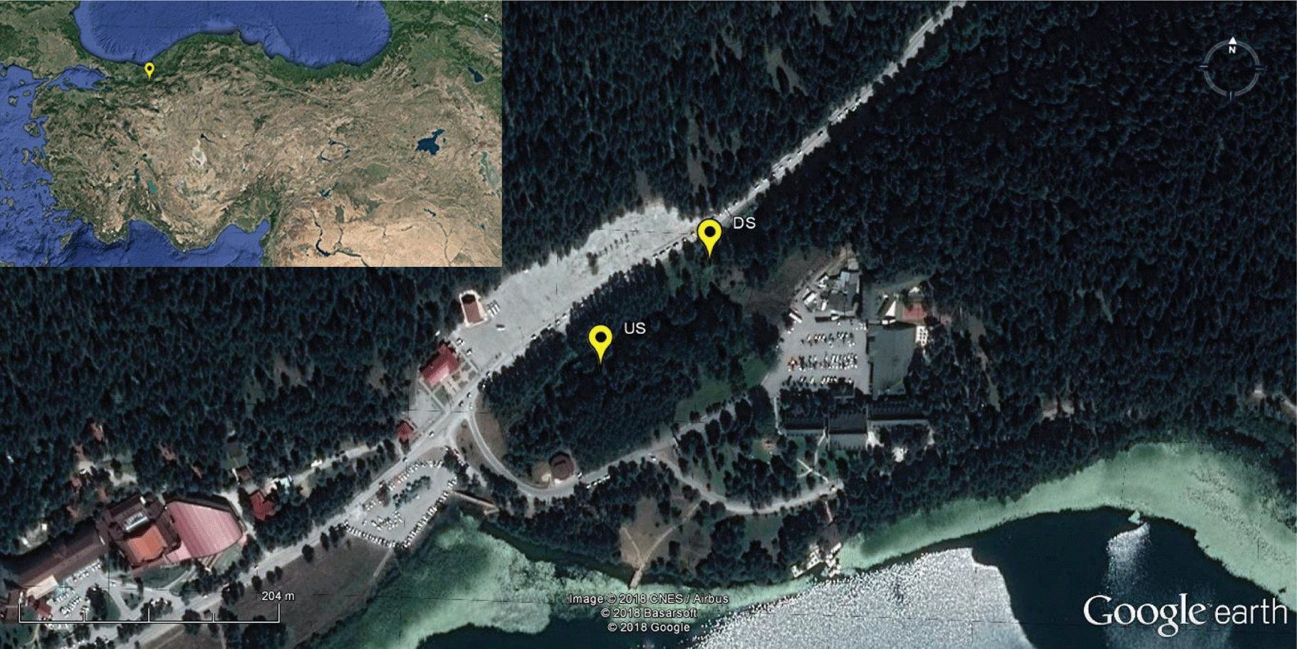
The Abant Creek is a forested stream, located in the province of Bolu in the western Black Sea region of Turkey, and rises from the Abant Lake at 1325 m elevation (Figure 1). According to the long-term meteorological data between 1927 and 2016, Bolu has a cool temperate climate with snowy winters and warm summers with cool nights. The mean annual temperature is 10.5 °C, the mean annual maximum and minimum temperature is 17.1 °C (max. 39.8 °C) and 4.5 °C (min. -34 °C), respectively, mean annual precipitation is 545.3 mm, the mean annual number of days with precipitation is 137.7, and mean annual sunshine hours are 65.6 h (total of the daily average of every month) [30]. Measurements of DO, water Temperature (Tw), and other environmental variables were carried out in a headwater (spring) reach of Abant Creek between August 2015 and December 2016. Upstream (US) and downstream (DS) coordinates (Lat., Long., in DD) of the reach are 40.612, 31.279, and 40.613, 31.280, reach slope and length are 0.0133 and 150 m, respectively (Figure 1).
Measurements of environmental variables
NEM was estimated by using a two-station method developed by Odum [16] for 17 months (between August 2015 and December 2016). DO and Tw measurements were performed at the upstream and downstream of the reach with one-minute intervals for at least 36 hours (2-3 days) by using oxygen data loggers (MiniDOT, PME, Vista, CA, USA). The reach length was selected as 150 m according to Bales and Nardi [31]. The data loggers were placed in protection cages throughout the measurements. While measuring DO and Tw, atmosphere pressure (Patm) was simultaneously measured by using data loggers (RHT50, Extech Instruments, USA). Water samples were collected at a 15-minute interval for two hours, while stream flow rate (Q), stream velocity (V), stream depth (D), and stream width (W) were measured by using an acoustic velocimeter (SonTek FlowTracker Handheld ADV, California, USA) at the time of both deployment and collection of the DO loggers in the reach. In water samples, pH and specific conductivity (SC) were measured by using a multi-parameter probe (Hach HQ40d portable meter, Hach Company, Loveland, CO, USA). Biochemical oxygen demand (BOD5) was measured by using a respirometric pressure system (WTW Oxitop IS6, Germany). Ortho-phosphate (orto-PO4-P), ammonium-nitrogen (NH4-N), and nitrate-nitrogen (NO3-N), chlorophyll a (chl-a) were measured by using a spectrophotometer (DR 5000 UV/VIS spectrophotometer, Hach Lange, Germany). Sampling days of the year (DOY) between August 2015 and December 2016 were 224-227, 244-246, 281-283, 316-318, 344-346 in 2015, and 13-15, 41-43, 77-79, 105-107, 140-142, 168-170, 195-197, 223-225, 265-267, 286-288, 314-316, 342-344 in 2016.
Calculations of NEM
NEM was calculated by using the following equations [28]:
Where Fr (t) is the reaeration flux (mg O2 reach-1 min-1) at time t, Deficitavg is the reach-averaged DO deficit (mg L-1) as DOsat (t) (DO saturation concentration) minus DO(t), K2(Tw) is the reaeration rate coefficient (min-1) at water temperature (Tw), Q is the stream flow rate (L s-1), Tt is travel time (min), and Cf is the unit conversion factor (one min = 60 s). K2 at Tw = 20°C was estimated using the equation by Owens, et al. [32] due to its suitability to the characteristics of the reaches sampled in this study.
Tw = 20 °C (0.12 ≤ D ≤ 3.35 m ve 0.03 ≤ V ≤ 1.52 m s-1) (2)
K2 at any Tw was calculated by using the following equation by Elmore and West [33]:
Where NEM (t) is the net metabolism flux (mg O2 reach-1 min-1) at time t, DOd(t) is downstream DO concentration (mg L-1) at time t, DOu(t-Tt) is upstream DO concentration (mg L-1) at time t-Tt.
High-frequency process model
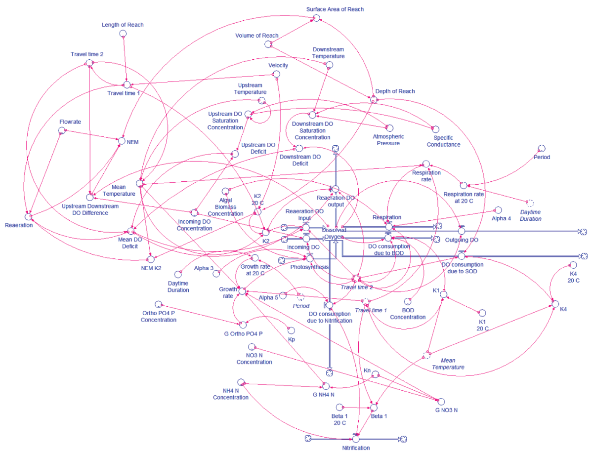
The model was developed by using the software STELLA to predict DO concentrations at one-minute intervals downstream of a 150-m headwater reach of Abant Creek. NEM was also estimated at each interval by using the two-station method in the model. The model was run for a day (including two nighttime and one daytime period) representing every month of the year. Measured data from January 2016 to December 2016, and from August 2015 to December 2015 were used for model calibration and validation, respectively. Model parameters were calibrated and validated according to mean absolute error (MAE) between measured and simulated (predicted) values of DO and NEM. The structure of the model was illustrated in Figure 2.
The equations used in the model are as follows (Brown & Barnwell, 1987):
Where α3 is the rate of DO production per unit of algal photosynthesis (mg O2 mg A-1), µ is the algal growth rate (min-1), α4 is the rate of DO uptake per unit of algae respired (mg O2 mg A-1), ρ is algal respiration rate (min-1), A is algal biomass concentration (mg L-1), K1 is carbonaceous deoxygenation (BOD) rate (min-1), LBOD is a concentration of carbonaceous BOD (mg L-1), K4 is sediment oxygen demand (SOD) rate (mg O2 m-2 min-1), D is a depth of stream (m), G(Ortho-PO4-P), G(NH4-N) and G(NO3-N) are monod expressions for phosphorus and nitrogen, respectively, KP and KN are half-saturation constants, α5 is the rate of DO uptake per unit of NH4-N oxidation (mg O2 mg N-1), α6 is the rate of DO uptake per unit of NO2-N oxidation (mg O2 mg N-1), β1 and β2 are nitrification rate coefficients (min-1) of NH4-N and NO2-N. NO2-N was neglected while the oxidation of NH4-N to NO3-N was in the nitrification process. So, α5 included α6 while β1 was including β2 in the model. The ratio of chl-a to algal biomass was assigned as 50 µg CHL-a/mg A [27].
Results and discussions
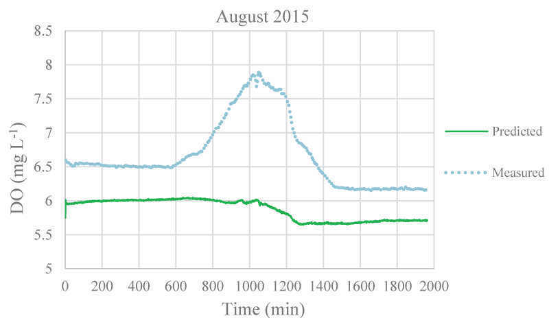
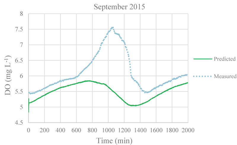
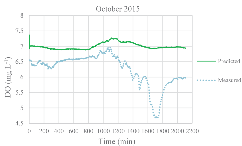
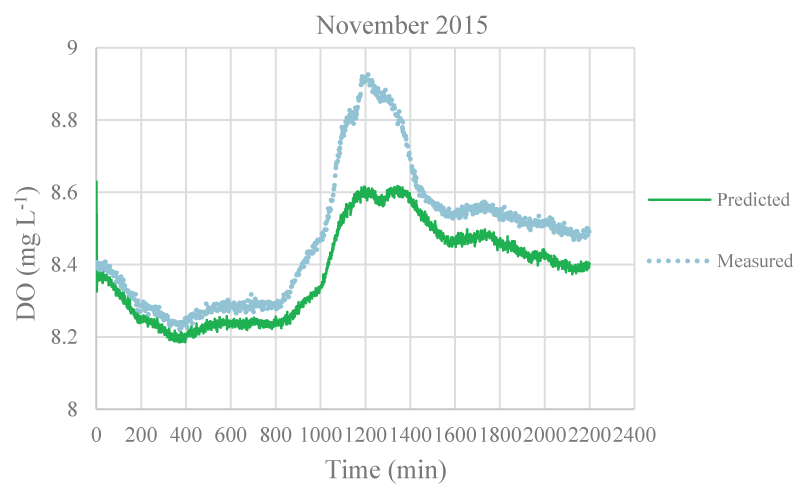
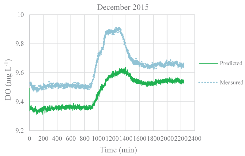
The mean monthly environmental variables measured and metabolism rates calculated between August 2015 and December 2016 were given in Table 1. The model coefficients were calibrated according to the ranges of Brown and Barnwell [27]. The calibrated coefficients, calibration, and validation results were given in Tables 2-4, respectively. MAEs between measured and simulated values of NEM ranged from 0.58 to 7.92 gr O2 m-2 day-1 and 1.3 – 7.78 gr O2 m-2 day-1 for calibration and validation, respectively. Figure 3-7 illustrated comparisons of one-minute measured and predicted DO concentrations during a day representing each month from August 2015 to December 2015 for validation. In the model, photosynthesis and respiration processes depend on only algal biomass. Aquatic plants and heterotrophs such as insects, and heterotrophic microorganisms living in the water were not included in these processes. Therefore, these deficiencies affected the DO predictions of the model.
According to calibration and validation results, differences (MAE and R2) between measured and predicted DO concentrations increased in July, August, September, October, November 2016, and August, September, and October 2015, respectively (Tables 3,4). In these months, the flow rate and velocity of the stream were very low (Table 1). Thus, high hydraulic retention durations might have enhanced photosynthesis and respiration processes by algae, aquatic plants, and heterotrophs in the water. Consequently, unavailable aquatic plant inputs in the model explain high differences between measured and predicted DO concentrations in these months. As is seen in Figures 3,4, the model was not able to simulate DO trends increasing in the daytime due to the causes/reasons mentioned above. In Figure 5, the measured DO concentration decreased suddenly. This might have been because of organic matters arising from rare leakages of the hotel sewage system around the study reached in a day (Figure 1). The model was not able to catch this fall in DO concentration since BOD input was constant for each interval (not temporal in a day) in the model. However, according to the rest of the months, the results showed that the model was successful and appeared to be promising in terms of high-frequency estimations of DO.
High-frequency values of NEM (as gr O2 m-2 min-1) were sensitive to DO differences with high flow rates even if there was a low difference (such as 0.1 mg L-1) between measured and predicted DO concentrations. Therefore, R2 between calculated and simulated NEMs was low (Tables 3,4).
Conclusion
The results demonstrated that algal biomass was inadequate for high-frequency modeling of DO oscillations in a daytime. Thus, aquatic plant inputs were also significant and should be considered for high-frequency DO modeling. BOD and nutrients (NH4-N, NO3-N, and orto-PO4-P) were measured in the two composite water samples taken at the time of deployment and collection of the DO loggers in the reach for 17 months. The means of two measurements of BOD and nutrients were assigned as constant inputs for each interval (dt = 1 min) in each month. Instead, all these inputs should be temporal (not constant) throughout the day for more accuracy.
Consequently, it can be said that aquatic plants in addition to the algal biomass, BOD, and nutrients are the main effective inputs. The model is modular and improvable to integrate more inputs (aquatic plants, etc.) so that much better predictions in high-frequency DO modeling can be obtained. Because it was very hard to estimate/predict DO concentrations and NEM values simultaneously within every minute during the day, the model was not able to predict observed values accurately (perfectly). However, acceptable predictions were obtained in this hard task. In future studies, the model can be modified and tested by using more inputs and data. Also, it can be applied under different conditions (instantaneous wastewater discharges, etc.) to predict DO and NEM variations.
Highlights
- The paper is the first study to include high-frequency modeling of both DO and NEM with one-minute intervals for the stream.
- The model was built in STELLA for the headwater reach of the Abant Creek in Bolu, Turkey.
- The model is simple and modular for high-frequency estimations of DO and NEM in the streams.
The authors thank Bolu Abant Izzet Baysal University for supporting the study. Also, the authors thank H. Fidan and E. Özalp for their help with field campaigns.
Funding information
This study was financially supported by the Scientific Research Projects Unit of Bolu Abant Izzet Baysal University (Grant No: BAP–2015.09.02.851).
- Davis JC. Minimal Dissolved Oxygen Requirements of Aquatic Life with Emphasis on Canadian Species: a Review. Journal of the Fisheries Research Board of Canada. 1975; 32(12): 2295-2332. https://doi.org/10.1139/f75-268.
- Dean TL, Richardson J. Responses of seven species of native freshwater fish and a shrimp to low levels of dissolved oxygen. New Zealand Journal of Marine and Freshwater Research. 1999; 33(1): 99-106. https://doi.org/10.1080/00288330.1999.9516860.
- Connolly NM, Crossland MR, Pearson RG. Effect of low dissolved oxygen on survival, emergence, and drift of tropical stream macroinvertebrates. Journal of the North American Benthological Society. 2004; 23(2): 251-270. https://doi.org/10.1899/0887-3593(2004)023<0251:EOLDOO>2.0.CO;2.
- Abowei JFN. Salinity, Dissolved Oxygen, pH and Surface Water Temperature Conditions in Nkoro River, Niger Delta, Nigeria. Advance Journal of Food Science and Technology. 2010; 2(1): 36-40.
- Hvitved-Jacobsen T. The impact of combined sewer overflows on the dissolved oxygen concentration of a river. Water Research. 1982; 16(7): 1099-1105. https://doi.org/10.1016/0043-1354(82)90125-7.
- Belanger SE. The effect of dissolved oxygen, sediment, and sewage treatment plant discharges upon growth, survival, and density of Asiatic clams. Hydrobiologia. 1991; 218: 113-126.
- Cooper CM. Biological Effects of Agriculturally Derived Surface Water Pollutants on Aquatic Systems-A Review. Journal of Environmental Quality. 1993; 22(3): 402-408. https://doi.org/10.2134/jeq1993.00472425002200030003x.
- Wang H, Hondzo M, Xu C, Poole V, Spacie A. Dissolved Oxygen Dynamics of Streams Draining an Urbanized and an Agricultural Catchment. Ecological Modeling. 2003; 160: 145–161. https://doi.org/10.1016/S0304-3800(02)00324-1.
- Morgan AM, Royer TV, David MB, Gentry LE. Relationships among nutrients, chlorophyll-a, and dissolved oxygen in agricultural streams in Illinois. J Environ Qual. 2006 May 31;35(4):1110-7. doi: 10.2134/jeq2005.0433. PMID: 16738396.
- Jankowski T, Livingstone DM, Bührer H, Forster R, Niederhauser P. Consequences of the 2003 European heat wave for lake temperature profiles, thermal stability, and hypolimnetic oxygen depletion: Implications for a warmer world. Limnology and Oceanography. 2006; 51(2): 815–819. https://doi.org/10.4319/lo.2006.51.2.0815.
- Stevens PW, Blewett DA, Casey JP. Short-term effects of a low dissolved oxygen event on estuarine fish assemblages following the passage of hurricane Charley. Estuaries and Coasts. 2006; 29(6):997-1003. https://doi.org/10.1007/BF02798661.
- Mulholland PJ, Houser JN, Maloney KO. Stream Diurnal Dissolved Oxygen Profiles as Indicators of in Stream Metabolism and Disturbance Effects: Fort Benning as a Case Study. Ecological Indicators.2005; 5: 243–252. https://doi.org/10.1016/j.ecolind.2005.03.004.
- Izagirre O, Agirre U, Bermejo M, Pozo J, Elosegi A. Environmental Controls of Whole-Stream Metabolism Identified From Continuous Monitoring of Basque Streams. Journal of the North American Benthological Society. 2008; 27(2): 252–268. https://doi.org/10.1899/07-022.1.
- Williamson CE, Dodds W, Kratz TK, Palmer M. Lakes and Streams as Sentinels of Environmental Change in Terrestrial and Atmospheric Processes. Frontiers in Ecology and the Environment. 2008; 6: 247–254. https://doi.org/10.1890/070140.
- Bernot MJ, Sobota DJ, Hall RO, Mulholland PJ, Dodds WK, Webster JR, Tank JL, Ashkenas LR, Cooper LW, Dahm CN, Gregory SV, Grimm NB, Hamilton SK, Johnson SL, McDowell WH, Meyer JL, Peterson B, Poole GC, Valett HM, Arango C, Beaulieu JJ, Burgin AJ, Crenshaw C, Helton AM, Johnson L, Merriam J, Niederlehner BR, O’Brien JM, Potter JD, Sheibley RW, Thomas SM, Wilson K. Inter-Regional Comparison of Land-Use Effects on Stream Metabolism. Freshwater Biology. 2010; 55: 1874–1890. https://doi.org/10.1111/j.1365-2427.2010.02422.x
- Odum HT. Primary Production in Flowing Waters. Limnology and Oceanography. 1956; 1: 102-117. https://doi.org/10.4319/lo.1956.1.2.0102.
- Kisi O, Akbari N, Sanatipour M, Hashemi A, Teimourzadeh K, Shiri J. Modeling of Dissolved Oxygen in River Water Using Artificial Intelligence Techniques. Journal of Environmental Informatics. 2013; 22(2): 92-101. DOI:10.3808/jei.201300248.
- Heddam S. Modeling hourly dissolved oxygen concentration (DO) using two different adaptive neuro-fuzzy inference systems (ANFIS): a comparative study. Environ Monit Assess. 2014 Jan;186(1):597-619. doi: 10.1007/s10661-013-3402-1. Epub 2013 Sep 21. PMID: 24057665.
- Zounemat-Kermani M, Seo Y, Kim S, Ghorbani MA, Samadianfard S, Naghshara S, Kim NW, Singh VP. Can Decomposition Approaches Always Enhance Soft Computing Models? Predicting the Dissolved Oxygen Concentration in the St. Johns River, Florida. Applied Sciences. 2019; 9(12): 2534. DOI: 10.3390/app9122534.
- Li J, Abdulmohsin HA, Hasan SS, Kaiming L, Al-Khateeb B, Ghareb MI, Mohammed MN. Hybrid soft computing approach for determining water quality indicator: Euphrates River. Neural Computing and Applications. 2019; 31(3): 827–837. DOI: 10.1007/s00521-017-3112-7.
- Ouma YO, Okuku CO, Njau EN. Use of Artificial Neural Networks and Multiple Linear Regression Model for the Prediction of Dissolved Oxygen in Rivers: Case Study of Hydrographic Basin of River Nyando, Kenya. Hindawi Complexity. 2020; 9570789. https://doi.org/10.1155/2020/9570789.
- Kisi O, Alizamir M, Docheshmeh Gorgij A. Dissolved oxygen prediction using a new ensemble method. Environ Sci Pollut Res Int. 2020 Mar;27(9):9589-9603. doi: 10.1007/s11356-019-07574-w. Epub 2020 Jan 10. PMID: 31925684.
- Lu H, Ma X. Hybrid decision tree-based machine learning models for short-term water quality prediction. Chemosphere. 2020 Jun;249:126169. doi: 10.1016/j.chemosphere.2020.126169. Epub 2020 Feb 11. PMID: 32078849.
- Asadollah SBHS, Sharafati A, Motta D, Yaseen ZM. River water quality index prediction and uncertainty analysis: A comparative study of machine learning models. Journal of Environmental Chemical Engineering. 2021; 9(1): 104599. https://doi.org/10.1016/j.jece.2020.104599.
- Dehghani R, Poudeh HT, Izadi Z. Dissolved oxygen concentration predictions for running waters with using hybrid machine learning techniques. Modeling Earth Systems and Environment. 2022; 8: 2599-2613. https://doi.org/10.1007/s40808-021-01253-x.
- Esen II, Rathbun RE. A Stochastic Model for Predicting the Probability Distribution of the Dissolved-Oxygen Deficit in Streams, Geological Survey professional paper; 913, Washington. 1976. https://doi.org/10.3133/ofr74224.
- Brown LC, Barnwell TO. The Enhanced Stream Water Quality Models QUAL2E and QUAL2E-UNCAS: Documentation and User Manual, EPA/600/3-87/007. Environmental Research Laboratory Office of Research and Development U.S. EPA, Athens, Georgia. 1987.
- Fang X, Stefan HG. Simulations of climate effects on water temperature, dissolved oxygen, and ice and snow covers in lakes of the contiguous U.S. under past and future climate scenarios. Limnology and Oceanography. 2009; 54(6): 2359-2370. https://doi.org/10.4319/lo.2009.54.6_part_2.2359.
- Feng ML, Sun T, Zhang LX, Shen XM. Net Ecosystem Metabolism Simulation by Dynamic Dissolved Oxygen Model in Yellow River Estuary, China. Procedia Environmental Sciences. 2012; 13: 807–817. https://doi.org/10.1016/j.proenv.2012.01.074.
- Turkish State Meteorological Service. (2017). Official Statistics. www.mgm.gov.tr.
- Bales JD, Nardi MR. Automated Routines for Calculating Whole-Stream Metabolism–Theoretical Background and User’s Guide: U.S. Geological Survey Techniques and Methods 4–C2, 33. Reston, Virginia. 2007. http://pubs.water.usgs.gov/tm4c2/.
- Owens M, Edwards RW, Gibbs JW. Some Reaeration Studies in Streams. International Journal of Air and Water Pollution. 1964; 8(8/9): 469-486.
- Elmore HL, West WF. Effect of Water Temperature on Stream Reaeration. Journal of the Sanitary Engineering Division. 1961; 87: 59–71. https://doi.org/10.1061/JSEDAI.0000360.
Article Alerts
Subscribe to our articles alerts and stay tuned.
 This work is licensed under a Creative Commons Attribution 4.0 International License.


 Save to Mendeley
